Managing AI model serving latency: a developer's guide
When a user submits a prompt to your GenAI application and waits two seconds for the first token, they notice. When that delay spikes to eight seconds during peak traffic, they leave. Managing AI model serving latency is not just a performance concern — it directly shapes user retention, infrastructure costs, and your team’s ability to scale confidently. This guide walks you through the full arc: measuring what actually matters, configuring your environment for observability, tuning your pipeline, surviving autoscaling events, and verifying that your changes hold up in production.
Table of Contents
- Understanding latency metrics and baseline measurement
- Preparing your serving environment: tools, metrics, and infrastructure setup
- Optimizing latency through model serving pipeline tuning
- Mitigating cold-starts and autoscaling latency spikes
- Verifying and troubleshooting AI serving latency in production
- Why focusing only on the model misses critical latency sources
- Explore MLflow’s AI platform for scalable, low-latency model serving
- Frequently asked questions
Key Takeaways
| Point | Details |
|---|---|
| Tail latency metrics | Monitor p90, p95, and p99 latency percentiles to understand the worst user experiences during AI model serving. |
| Baseline profiling | Establish latency baselines with isolated model benchmarks using tools like trtexec before system-level optimization. |
| Integrated observability | Combine inference time, queue size, batching, and cold-start metrics for accurate latency diagnostics. |
| Pipeline tuning | Use cache-aware routing, continuous batching, and smart scheduling to reduce serving latency beyond model improvements. |
| Cold start mitigation | Address latency spikes from autoscaling zero instances with keep-alives and adapter size optimizations. |
Understanding latency metrics and baseline measurement
To reduce serving latency effectively, you must first understand how to measure and benchmark it accurately. Not all latency metrics tell the same story, and optimizing for the wrong one can leave your worst user experiences untouched.
Tail latency (p90, p95, p99) is the metric that most closely reflects what real users experience. Average latency can look healthy while your p99 sits at 12 seconds. Tracking tail latency paired with pipeline metrics like queue depth and batching helps spot regressions before GPU utilization shows anomalies. If you are only watching mean response time, you are watching the wrong number.
Time to First Token (TTFT) deserves its own dashboard. For streaming applications, TTFT is the latency users feel most acutely. A model that generates tokens quickly but takes three seconds to start feels broken, even if its throughput is excellent. Track TTFT separately from total generation time.
Here are the core metrics to instrument from day one:
- TTFT (Time to First Token): critical for streaming UX
- Time per output token (TPOT): measures generation throughput
- Queue depth: requests waiting for an available worker
- Batch size: actual vs. configured maximum
- Cold-start frequency: how often instances initialize from zero
- p90/p95/p99 latency: tail behavior across the request distribution
For baseline measurement, NVIDIA recommends establishing a latency/throughput baseline using "trtexec` with the model run in isolation, then profiling with Nsight Systems to find bottlenecks beyond raw inference latency. This two-step approach separates what the model itself costs from what your pipeline adds around it.
| Metric | What it reveals | Tool |
|---|---|---|
| p99 latency | Worst-case user experience | Prometheus, Grafana |
| TTFT | Streaming responsiveness | Custom instrumentation |
| Queue depth | Scheduling pressure | Serving framework metrics |
| GPU utilization | Compute saturation (not a scaling trigger) | NVIDIA DCGM |
| Cold-start rate | Infrastructure readiness | Cloud provider metrics |
Pro Tip: Run trtexec with --percentile=99 to capture p99 latency during your baseline benchmark. This gives you a reproducible number to compare against after every pipeline change.
Good model serving observability starts at this layer. Before you touch a single configuration knob, know your baseline tail latency, your TTFT distribution, and your queue behavior under load. Everything else builds from there.
Preparing your serving environment: tools, metrics, and infrastructure setup
With baselines and metrics defined, the next step is to configure your environment to track and respond to latency effectively. This is where many teams underinvest, and it costs them later when a regression surfaces in production with no clear cause.
Integrated observability tracking inference time, tail latency, queue depth, and cold-start signals is essential to quickly narrow down causes of latency degradation. Set up end-to-end tracing before you deploy to production, not after your first incident. The AI observability tracing techniques you put in place now will save hours of guesswork later.

Infrastructure choices matter more than most teams realize. Sticky routing, which sends requests from the same session or prefix to the same replica, allows KV cache reuse and can cut TTFT dramatically for multi-turn conversations. If your load balancer uses pure round-robin, you are throwing away free latency gains. Choose infrastructure that supports session-aware routing from the start.
Serverless or autoscaled hosting often causes cold-start latency spikes affecting TTFT, which must be accounted for in system design. Plan for this explicitly. If your serving platform scales to zero during low-traffic periods, your first request after a quiet window will pay the full initialization cost.
Key environment configuration checklist:
- Enable distributed tracing on every inference endpoint
- Export queue depth and batch size as real-time metrics
- Configure autoscaling triggers on queue depth, not GPU utilization
- Set up alerting on p95 and p99 thresholds, not just average latency
- Test cold-start behavior explicitly during load testing
- Use sticky routing where KV cache reuse is possible
Your serving platform infrastructure should expose these signals natively. If it does not, instrument them yourself before you go further. You cannot manage what you cannot see.
Pro Tip: During load testing, deliberately trigger a scale-to-zero event and measure the resulting TTFT spike. Document this number. It becomes your cold-start SLA baseline and informs decisions about minimum replica counts.
Optimizing latency through model serving pipeline tuning
Having prepared your environment, you can now execute pipeline tuning techniques to reduce serving latency effectively. This is where the biggest gains typically live, and also where the most common mistakes happen.
- Switch to continuous batching. Fixed batching holds requests until a batch fills, adding queuing delay for every request. Continuous batching processes tokens as they complete, reducing head-of-line blocking and improving both throughput and tail latency simultaneously.
- Deploy PagedAttention-based serving. vLLM’s tail latency improvements stem from PagedAttention techniques and continuous batching, resulting in 2.2x to 2.3x better p99 latency and TTFT over alternative approaches. If you are not using a PagedAttention-based engine, this is your highest-leverage change.
- Implement cache-aware routing. Cache-aware routing avoids redundant prefill, reducing latency dramatically compared to round-robin, by sending requests to replicas holding relevant context. For applications with shared system prompts or multi-turn sessions, this can eliminate the prefill cost entirely on subsequent requests.
- Align dynamic batching with your optimization profile. If your model was compiled with TensorRT at a specific batch size, serving requests at a different batch size forces recompilation or suboptimal execution. Match your runtime batch configuration to your model’s optimization profile.
- Scale on queue depth, not GPU utilization. GPU utilization lags behind actual demand, especially for memory-bandwidth-bound decoding workloads. By the time utilization spikes, your queue is already backing up. Use the inference routing best practices that treat queue depth as the primary autoscaling signal.
| Technique | Latency impact | Complexity |
|---|---|---|
| Continuous batching | High (reduces head-of-line blocking) | Low |
| PagedAttention (vLLM) | Very high (2x+ p99 improvement) | Medium |
| Cache-aware routing | High (eliminates prefill for cached prefixes) | Medium |
| TensorRT compilation | Medium (faster per-token compute) | High |
| Queue-based autoscaling | High (prevents tail latency spikes) | Low |
Pro Tip: When evaluating batching and memory techniques, measure p99 latency at your target concurrency level, not just average latency at low load. Optimizations that look great at 10 concurrent requests often behave differently at 200.
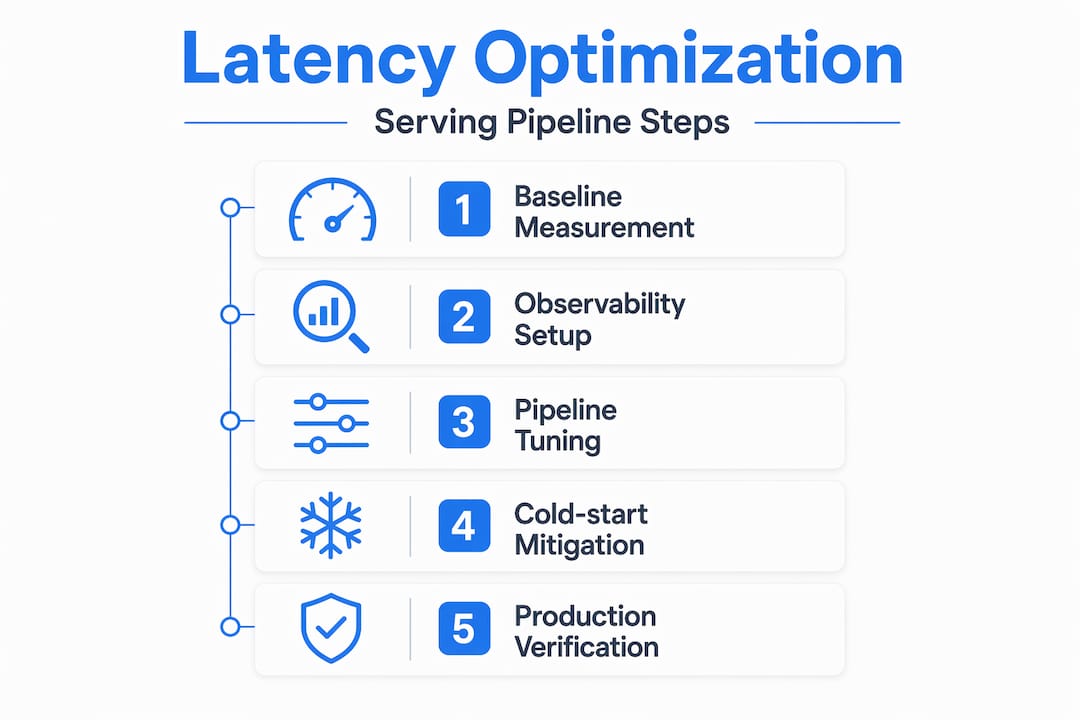
Mitigating cold-starts and autoscaling latency spikes
In addition to tuning pipeline steps, mitigating cold starts and autoscaling spikes is critical to maintaining low latency during traffic fluctuations. This is the category of latency that surprises teams most in production.
Cold starts cause latency spikes primarily in Time to First Token, typically a few hundred milliseconds for LoRA adapter loads after scaling to zero. For applications where TTFT is a core UX metric, even a 300ms spike on the first request of a session is noticeable. For applications with strict SLAs, it can be a violation.
The sources of cold-start latency break down as follows:
- Model weight loading: the base model must transfer from storage to GPU memory
- LoRA adapter initialization: fine-tuned adapters load on top of base weights
- KV cache allocation: memory pages must be allocated before generation begins
- Container startup: the serving process itself must initialize
Autoscaling based on GPU metrics alone can be too slow. Queue depth metrics per replica enable proactive scaling to avoid tail latency regressions. The goal is to scale before requests start queuing, not after they have already waited.
Practical mitigation strategies:
- Set a minimum replica count of at least 1 to avoid full scale-to-zero events for latency-sensitive endpoints
- Use periodic keep-alive requests (a lightweight ping every 30 to 60 seconds) to prevent instance hibernation
- Pre-load LoRA adapters at startup rather than loading them on first request
- Monitor serverless deployment latency separately from steady-state latency in your dashboards
Pro Tip: If you must allow scale-to-zero for cost reasons, implement a warm-up endpoint that fires immediately after a new instance starts. This pre-allocates KV cache memory and loads adapters before the first real user request arrives.
Verifying and troubleshooting AI serving latency in production
After implementing optimization and mitigation steps, verifying latency behavior in production ensures sustained performance and rapid diagnosis of new issues.
Average latency is a trap. A deployment that improves mean response time by 40% while worsening p99 by 20% is a regression for your worst-affected users. Always verify improvements by comparing tail latency percentiles before and after each change.
Distributed tracing with tools like OpenTelemetry enables detailed visibility of each inference step, unraveling latency spikes that average metrics hide. A trace that spans tokenization, queue wait, prefill, decode, and detokenization tells you exactly where time is going on a per-request basis.
Here is a verification workflow we recommend for every optimization cycle:
- Record p90, p95, and p99 latency plus TTFT before making any change
- Deploy the change to a canary slice (10 to 20% of traffic)
- Run a load test at your target concurrency level against the canary
- Compare tail latency percentiles and TTFT between canary and baseline
- Check queue depth behavior under the same load profile
- Monitor for at least 24 hours before full rollout to catch time-of-day effects
For ongoing production monitoring, configure alerts on these signals:
- p99 latency exceeds your SLA threshold for more than 60 seconds
- Queue depth per replica exceeds your target maximum
- TTFT spikes more than 2x the baseline for any 5-minute window
- Cold-start rate increases following a deployment
“The goal of production latency verification is not to prove that your optimization worked once. It is to build confidence that it holds under the full range of traffic patterns your system will encounter.”
AI model tracing with MLflow gives you the per-request visibility to distinguish between a model-side slowdown and a pipeline-side regression. Without that granularity, you are guessing. With it, you can resolve most latency incidents in minutes rather than hours.
Pro Tip: Use tail-based sampling in your tracing setup. Capture 100% of requests that exceed your p99 threshold and 100% of errors, but sample routine fast requests at 1 to 5%. This keeps trace volume manageable while ensuring you never miss a slow request.
Why focusing only on the model misses critical latency sources
Here is the uncomfortable truth most latency optimization guides skip: the model is rarely the bottleneck. Teams spend weeks squeezing inference time, compiling with TensorRT, and quantizing weights, then discover that CPU preprocessing and tokenization are adding more latency than the GPU step they just optimized.
NVIDIA frames serving latency as pipeline friction, where CPU preprocessing, synchronization, and scheduling often dominate over raw model inference latency. This is not a niche edge case. It is the default situation in most production serving stacks, and it only becomes visible through system-level profiling with tools like Nsight Systems.
The same pattern appears in autoscaling decisions. Databricks’ guidance highlights the central role of queue dynamics and concurrency provisioning rather than GPU utilization alarms in managing tail latency in production LLM serving. Teams that scale on GPU utilization are reacting to a lagging indicator. By the time utilization crosses a threshold, the queue has already grown and tail latency has already spiked.
We have seen this play out repeatedly. A team optimizes their model to run 30% faster in isolation, deploys it, and sees no improvement in production p99 latency. The reason: their queue was the bottleneck, not the model. Adding concurrency, not a faster model, was what they actually needed.
Effective latency management is a cross-layer problem. It requires coordinated tooling across the model, the serving framework, the routing layer, and the infrastructure. Advanced latency observability that spans all of these layers is not optional. It is the only way to know where time is actually going.
The teams that consistently maintain low tail latency in production are not the ones with the fastest models. They are the ones with the clearest visibility into their full serving stack.
Explore MLflow’s AI platform for scalable, low-latency model serving
Managing AI model serving latency across all of these layers — profiling, pipeline tuning, cold-start mitigation, and continuous verification — requires tooling that spans the full serving lifecycle. MLflow is built for exactly this challenge.
The MLflow GenAI engineering platform gives your team production-grade observability, deep tracing of every inference step, and a centralized AI Gateway for serving that supports cache-aware routing and queue-based autoscaling. With MLflow AI observability tools, you can track tail latency, TTFT, and queue depth in a single pane, and connect trace data directly to the requests that caused your worst latency events. If your team is serious about reducing AI latency in production GenAI applications, MLflow gives you the infrastructure to do it systematically.
Frequently asked questions
What is tail latency and why is it important in AI model serving?
Tail latency measures the higher percentiles of request delays (p95, p99), representing the slowest requests your users experience. Tail latency captures delays many users experience and is key for spotting regressions early, making it a more reliable quality signal than average response time.
How does profiling with tools like trtexec and Nsight Systems help reduce latency?
trtexec benchmarks isolated model inference performance to establish a clean baseline, while Nsight Systems reveals CPU and GPU pipeline bottlenecks beyond the model itself. Use trtexec for baseline and Nsight Systems for system-level profiling to find CPU bottlenecks and idle GPU time, enabling targeted optimizations that address the actual source of end-to-end latency.
What causes cold start latency spikes in serverless AI model serving?
Cold start spikes occur when autoscaled instances scale to zero and must reload model weights and LoRA adapters before serving the first request. Cold starts happen when workloads scale to zero and weights are reloaded, causing TTFT spikes primarily, typically in the range of a few hundred milliseconds.
Why is queue depth a better scaling metric than GPU utilization for LLM serving?
Queue depth directly measures how many requests are waiting, making it a leading indicator of tail latency degradation. Queue depth per replica signals sudden traffic surges sooner than GPU utilization, enabling proactive scaling to avoid tail latency regressions, especially in memory-bandwidth-bound decoding workloads where GPU utilization can appear stable even as queues grow.