2 posts tagged with "AI deployment strategies"

The most cost-effective and SLO-safe way to scale production inference is a system-level combination of disaggregated serving, topology-aware autoscaling, and model/runtime optimizations matched to your workload profile. No single lever gets you there alone.

Your next 7 days:

• SLO inventory: Pull p95 and p99 TTFT (time-to-first-token) and tokens/sec from your current serving stack. If you don't have those metrics yet, that gap is your first problem.
• Workload profile check: Classify traffic as low-latency user-facing, high-throughput batch, or agentic/multi-call. Each drives a different infra decision tree.
• Cold-start baseline: Measure how long a cold pod takes to serve its first token under realistic load. That number tells you whether warm-pool pre-warming or multicast-based distribution is worth the engineering investment.

For steady high-throughput workloads, quantization plus disaggregated prefill/decode separation reduces TCO fastest. For bursty or agentic traffic, topology-aware autoscaling and cold-start mitigation are the higher-priority levers.

Key Takeaways​

Scaling AI inference infrastructure requires a system-level approach: disaggregated serving, topology-aware autoscaling, and model optimizations matched to workload profile deliver the best combination of latency control and TCO reduction.

Table of Contents​

• Why scaling AI inference is a system-level problem
• How to choose between cloud, bare-metal Kubernetes, and purpose-built inference stacks
• What distributed inference strategy should you use?
• How do you autoscale inference pools safely and cost-effectively?
• Which model optimizations reduce inference cost the most?
• Hardware and network choices that actually affect scale
• How to deploy and operate inference fleets with Kubernetes
• How to validate that your scaling choices meet SLOs in production
• What does FaaScale's PipeCast research mean for cold-start scaling?
• Stage-by-stage validation checklist: pilot to production
• Cost optimization and capacity planning for inference workloads
• Recommended architectures and a 30/60/90-day rollout plan
• What platform teams actually get wrong when scaling inference
• Mlflow fits naturally into an inference-scaling journey
• Sources

Why scaling AI inference is a system-level problem​

Adding GPUs without addressing the rest of the stack is one of the most common and expensive mistakes in production inference. The bottleneck shifts: you provision more compute, and suddenly the interconnect saturates, or the KV cache spills to host memory, or the orchestration layer can't place gang-scheduled pods fast enough. Scaling AI infrastructure from chip to cluster is fundamentally a multi-layer problem, and each layer has its own failure mode.

Think of the stack as five interdependent tiers:

1. Chip/device layer: GPU compute and on-device HBM (e.g., 80 GB on an H100 SXM). This is where matrix multiplications happen and where memory bandwidth limits sequence length.
2. Node layer: NVLink/NVSwitch fabric connecting GPUs within a node. NVSwitch-based nodes (DGX H100) deliver up to 900 GB/s all-reduce bandwidth, which is why tensor parallelism within a node is far cheaper than across nodes.
3. Rack/cluster layer: InfiniBand or high-speed Ethernet (e.g., NVIDIA Spectrum-X) connecting nodes. Cross-node collectives via NCCL are bandwidth-constrained here; topology mismatches cause head-of-line blocking.
4. Storage and host-memory layer: CPU RAM and NVMe SSDs used for KV cache offload, model weight staging, and checkpoint storage. Slow storage here directly inflates cold-start latency.
5. Orchestration and software layer: Kubernetes operators, serving frameworks (vLLM, TensorRT-LLM), and load balancers. Placement errors at this layer waste the hardware investment below it.

Microsoft's engineering notes on hyperscale AI datacenters confirm that interconnect, topology, and system-level design from chip to cluster are the primary constraints when scaling inference beyond a single node.

Three workload profiles and what they demand​

Low-latency user-facing LLMs (chatbots, copilots): p99 TTFT under 500 ms is a typical SLO. These workloads need fast prefill, warm decode pools, and KV cache locality. Disaggregated serving shines here because you can scale prefill and decode independently.

High-throughput batch inference (vision models, recommender systems, offline scoring): throughput per dollar matters more than tail latency. You can tolerate higher p99 in exchange for better GPU utilization. Continuous batching and larger batch sizes are the primary levers.

Agentic and multi-call pipelines (LLM chains, tool-use agents): these generate many short requests in sequence, often with shared context. KV cache reuse across calls is critical; cold-start overhead compounds across every hop in the chain.

Why percentiles matter more than averages​

A p50 TTFT of 200 ms looks fine in a dashboard. A p99 of 4 seconds means 1 in 100 users waits four seconds for the first token, which is a product failure for real-time applications. SLOs must be defined at p95 and p99, not at mean or median, because tail latency is where user experience breaks and where autoscaler triggers need to fire.

How to choose between cloud, bare-metal Kubernetes, and purpose-built inference stacks​

The right infrastructure baseline depends on your traffic pattern, data residency requirements, and team's operational maturity. There is no universally correct answer, but the decision tree is short.

Cloud (AWS, GCP, Azure GPU instances) wins for bursty or experimental workloads. You pay per hour, avoid capital expenditure, and can spin up a new model version in minutes. Cold-start latency is higher because GPU instances take time to provision, but managed autoscaling handles demand spikes without a dedicated ops team. The cost premium over on-prem is real at sustained load, but for teams still iterating on model architecture, the flexibility outweighs it. Practical architecture guidance consistently recommends cloud for burst and experimentation, on-prem or hybrid for sustained high-volume inference.

Bare-metal Kubernetes wins for steady, high-volume inference with strict data residency or compliance requirements. You own the hardware, so you control the NVLink topology, the NCCL configuration, and the network fabric. TCO at scale is lower than cloud, but you carry the operational burden: hardware failures, driver upgrades, capacity planning, and rack-level networking. Teams running millions of inference requests per day on a predictable traffic curve typically see better economics here within 12–18 months of sustained load.

Purpose-built inference stacks (managed inference endpoints, disaggregated serving platforms) make sense at very large scale where the engineering cost of building and maintaining a custom orchestration layer exceeds the cost of a managed service. These stacks often bundle KV-aware routing, disaggregated prefill/decode, and autoscaling out of the box.

Decision checklist:

• Bursty traffic + no data residency constraint + team < 5 infra engineers: start on cloud managed GPU instances.
• Steady traffic > 10M requests/day + data residency or compliance requirement: invest in bare-metal Kubernetes with topology-aware operators.
• Very large scale (100B+ parameter models, multi-tenant serving) + dedicated infra team: evaluate purpose-built disaggregated stacks.
• Hybrid: use cloud for burst overflow and on-prem for the steady baseline. Reserve capacity contracts on cloud reduce the cost premium for predictable burst windows.

Cost profile comparison:

• Cloud: high opex, low capex, elastic. Spot/preemptible instances cut GPU costs by 60–70% for fault-tolerant batch workloads, but are unsuitable for latency-sensitive serving without fallback pools.
• Bare-metal: high capex, low opex at scale, fixed capacity. Requires 12–18 months to amortize hardware.
• Purpose-built stacks: variable opex, often usage-based. Multi-tenancy isolation is typically stronger out of the box.

Cold-start behavior: Cloud instances cold-start in minutes (instance provisioning + model loading). Bare-metal Kubernetes with pre-warmed node pools cold-starts in seconds to tens of seconds (pod scheduling + weight loading). Purpose-built stacks vary widely; some use multicast-based model distribution to cut cold-start to sub-second ranges.

What distributed inference strategy should you use?​

The right distributed strategy depends on model size, sequence length, your latency SLO, and whether you're optimizing for throughput or cost. Picking the wrong one wastes GPU memory and adds unnecessary communication overhead.

The short answer: use tensor parallelism within a node when a model's layers don't fit in a single GPU's HBM. Use pipeline parallelism across nodes when the full model doesn't fit in one node. Use context parallelism for very long sequences (100K+ tokens). Use disaggregated serving to separate prefill from decode when you need independent scaling of those two phases.

Distributed strategy comparison​

TensorRT 11.0's multi-device inference primitives (IDistCollectiveLayer) document the communication trade-offs between AllGather KV, Ring Attention, and DeepSpeed Ulysses patterns for long-context and multi-device inference. Ring Attention distributes attention computation across devices with O(1) communication per step, while Ulysses (from DeepSpeed) uses all-to-all communication to partition heads across devices, which is more efficient at smaller sequence counts but less so at very long contexts.

Disaggregated prefill/decode in practice​

NVIDIA Dynamo's disaggregated serving architecture separates prefill workers (which process the input prompt) from decode workers (which generate tokens one step at a time). This matters because prefill is compute-bound and bursty, while decode is memory-bandwidth-bound and steady. Mixing them on the same GPU pool means one phase always starves the other.

In a disaggregated setup, a KV-aware router directs incoming requests to a prefill pool, which computes the KV cache and transfers it to a decode pool. The decode pool then generates tokens without re-running prefill. Dynamo also supports KV block offload to storage tiers, which lets you serve more concurrent sessions than GPU HBM alone would allow.

When to prefer context parallelism: long-context media transcription, legal document analysis, or vision workloads where sequences exceed 32K tokens. Ring Attention or Ulysses patterns distribute the attention computation across GPUs, keeping per-device memory within bounds.

When to prefer tensor/pipeline parallelism: model-sharded scenarios where a 70B or 405B parameter model must be split across devices. Tensor parallelism within a node (NVLink) is always preferred over pipeline parallelism across nodes (InfiniBand) when the model fits, because intra-node bandwidth is an order of magnitude higher.

Pro Tip: *For KV cache reuse in agentic pipelines, prefix caching (storing KV blocks for common prompt prefixes) can eliminate redundant prefill computation across tool-use chains. vLLM's prefix caching and Dynamo's KV block manager both support this pattern.

How do you autoscale inference pools safely and cost-effectively?​

Autoscale by SLO metrics, not by CPU or memory utilization. CPU and memory are lagging indicators for GPU inference workloads. By the time CPU utilization spikes, your decode pool has already been queuing requests for seconds.

Metrics to collect and alert on​

1. p95/p99 TTFT: the primary SLO metric for user-facing LLMs. Alert when p99 exceeds your SLO threshold for more than 60 seconds.
2. Queue depth per pool: number of requests waiting for a prefill or decode slot. A rising queue depth is the earliest signal of capacity pressure.
3. Tokens/sec per GPU: throughput efficiency. Declining tokens/sec with stable request rate indicates memory pressure or KV cache thrashing.
4. Cost per 1,000 tokens: the financial SLO. Track this per model version to catch regressions after deployments.
5. KV cache hit rate: for agentic or multi-turn workloads. A hit rate below 30% suggests prefix caching is misconfigured or cache capacity is too small.

A 2025 arXiv study on cloud AI inference scalability shows that hybrid ML-based autoscaling combining deep learning demand forecasting with reinforcement learning for allocation outperforms classical round-robin and least-connections approaches in dynamic cloud inference environments, improving both utilization and response time.

Autoscaler design patterns​

Topology-aware gang scheduling places all pods in a parallelism group on GPUs within the same NVLink domain or rack before scheduling across nodes. Kubernetes operators like those in the ai-dynamo/dynamo project (Grove patterns) implement topology-aware placement and declarative startup ordering to prevent partial-gang cold-starts.

SLO-driven planner: profile your prefill and decode pools separately. When p99 TTFT rises, scale the prefill pool first (it's usually the bottleneck for bursty traffic). When tokens/sec per GPU drops, scale the decode pool. Treating them as a single autoscaling unit is a common mistake that leads to over-provisioning one pool while the other starves.

Cold-start mitigation​

Cold-start in a GPU inference pod has two components: pod scheduling time and model weight loading time. Pod scheduling is a Kubernetes problem; model weight loading is a storage and distribution problem.

Practical mitigations:

• Warm pools: keep a small number of pre-warmed pods (weights loaded, no traffic) to absorb sudden bursts without full cold-start latency.
• Model pre-warming: load weights into GPU HBM before the pod is marked ready. This adds startup time but eliminates the first-request penalty.
• Multicast/PipeCast (research): FaaScale's PipeCast approach multicasts model blocks to multiple workers simultaneously and begins inference on partially-received blocks. This is covered in depth in the research extension section below.

For AI service load management, the combination of warm pools and topology-aware scheduling covers most production cold-start scenarios without requiring experimental multicast infrastructure.

Pro Tip: Under token burst conditions (e.g., a user submitting a 10,000-token prompt), protect your decode pool with adaptive admission control. Set a maximum queue depth threshold and return a 429 with a Retry-After header rather than letting the decode pool queue grow unbounded. Request shaping at the gateway layer (token-bucket rate limiting per tenant) prevents one tenant's burst from degrading p99 for all others.

Which model optimizations reduce inference cost the most?​

Quantization and KV caching are the highest-ROI levers for inference TCO without major accuracy loss, provided you validate correctness before rolling out to production. Everything else is secondary until those two are in place.

Quantization:

• FP16: the standard baseline for most LLM serving. Cuts memory footprint roughly in half versus FP32 with negligible accuracy loss on most tasks.
• FP8: supported on H100 and newer GPUs. Reduces HBM usage further and increases throughput on compute-bound layers. Accuracy impact is model-dependent; always run your eval suite before promoting to production.
• INT8 (weight-only or activation quantization): effective for memory-bandwidth-bound decode. Tools like TensorRT's quantization toolkit and vLLM's AWQ/GPTQ integrations make this accessible. Expect 1–3% accuracy degradation on complex reasoning tasks; measure it on your specific workload.

Pruning and distillation: structured pruning (removing entire attention heads or MLP blocks) reduces FLOPs but requires fine-tuning to recover accuracy. Knowledge distillation trains a smaller student model on the larger model's outputs. Both are higher-effort than quantization and are worth pursuing only after quantization is fully exploited.

Operator fusion: fusing attention, layer norm, and activation operations into a single CUDA kernel reduces memory round-trips and kernel launch overhead. TensorRT and vLLM both apply operator fusion automatically; the main action item is to verify that your model's custom ops are compatible with the fusion pass.

KV cache strategies:

• Paged KV caching (vLLM's core innovation): allocates KV cache in fixed-size pages rather than contiguous blocks, eliminating fragmentation and enabling higher GPU utilization.
• Tiered KV offload: spill less-recently-used KV blocks to CPU RAM or NVMe. Dynamo's KV block manager supports this. Latency increases for cache misses, so set eviction policies based on your session length distribution.
• Prefix caching: store KV blocks for common prompt prefixes. Particularly effective for agentic pipelines where system prompts are shared across thousands of requests.

Validation and rollout gating:

Before promoting any optimization to production, run an A/B test with shadow traffic. Compare p95/p99 TTFT, tokens/sec, and accuracy metrics (BLEU, task-specific evals, or LLM-as-a-Judge scores) between the baseline and optimized variant. Track inference speed improvements per model version so regressions are caught before they reach 100% traffic.

Hardware and network choices that actually affect scale​

Interconnect and topology often limit scale more than raw GPU FLOPs. A cluster of H100s with misconfigured NCCL or insufficient InfiniBand bandwidth will underperform a smaller, well-connected cluster.

GPU selection checklist:

• HBM capacity: match to your largest model shard. An H100 SXM has 80 GB HBM3; an H200 has 141 GB. For a 70B parameter model in FP16, you need ~140 GB, which means two H100s minimum for tensor parallelism.
• NVLink generation: H100 NVLink 4.0 delivers 900 GB/s bidirectional bandwidth per GPU. This is the threshold where intra-node tensor parallelism becomes practical for large models.
• CPU and host memory: size host RAM to hold at least one full model copy for KV offload and weight staging. 512 GB per node is a reasonable floor for 70B-class models.
• Local NVMe: fast local SSDs (NVMe Gen4/Gen5) reduce model loading time from storage. A 70B FP16 model is ~140 GB; loading from NVMe at 7 GB/s takes about 20 seconds versus minutes from network storage.

Network topology:

Within a node, NVLink/NVSwitch is the right fabric for tensor parallelism. NVIDIA's telemetry documentation for Spectrum-X confirms that topology-aware collectives via NCCL materially affect multi-GPU and multi-node throughput, and that scheduling decisions should reflect the physical topology.

Across nodes, InfiniBand HDR/NDR (200–400 Gb/s per port) is the standard for high-performance multi-node inference. For pipeline parallelism across nodes, the inter-node bandwidth determines pipeline bubble size. For tensor parallelism across nodes (generally avoid this), you need near-NVLink bandwidth, which InfiniBand does not provide.

NCCL handles collective communication (AllReduce, AllGather, Broadcast) and automatically selects the fastest path based on topology. Set NCCL_TOPO_FILE to your cluster's topology XML to prevent NCCL from making suboptimal routing decisions in heterogeneous environments.

Procurement and cost amortization:

• On-prem GPU servers: plan for 3–5 year amortization. Power and cooling add 30–50% to hardware TCO in most US data centers; factor this into your cloud vs on-prem comparison.
• Rack density: H100 DGX nodes draw 10.2 kW each. A 42U rack can hold 4–6 DGX nodes, requiring 40–60 kW of power delivery and liquid cooling in most modern deployments.
• Cloud reserved instances: 1-year or 3-year reservations on GPU instances reduce on-demand pricing by 30–60% and are appropriate for the steady-state baseline of a hybrid architecture.

How to deploy and operate inference fleets with Kubernetes​

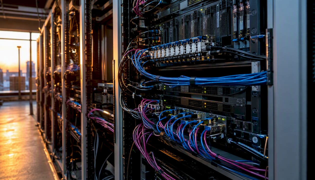
Topology-aware orchestration and explicit startup ordering reduce cold-start failures and placement errors more than any other operational change at the Kubernetes layer. Without them, gang-scheduled pods land on suboptimal nodes, NCCL performance degrades, and partial-gang failures cascade.

Deployment playbook​

Operator and CRD patterns: use a Kubernetes operator that understands GPU topology. The ai-dynamo/dynamo project provides operator patterns (Grove-style) that implement topology-aware gang scheduling and declarative startup ordering via CRDs. A typical CRD spec declares the parallelism group size, the required NVLink domain, and the startup dependencies between components (KV cache service, prefill pool, decode pool).

Startup ordering: prefill pools depend on the KV cache service being ready. Decode pools depend on the prefill pool being healthy. Expressing these dependencies explicitly in your operator (via readiness gates or init containers) prevents the common failure mode where a decode pod starts accepting traffic before its prefill counterpart is ready, causing request timeouts.

A minimal startup sequence for a disaggregated serving stack:

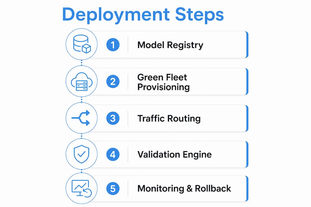
1. KV cache service (storage backend) → Ready
2. Prefill pool (N pods, topology-pinned) → All pods Ready
3. Decode pool (M pods, topology-pinned) → All pods Ready
4. Router/load balancer → Ready, begins accepting traffic

Multi-tenancy and isolation: use Kubernetes namespaces with resource quotas (GPU limits, memory limits) to isolate tenants. For strict isolation (e.g., different compliance boundaries), use separate node pools per tenant with node selectors and taints. For soft multi-tenancy (shared infrastructure, logical isolation), priority classes and preemption policies prevent one tenant's batch job from evicting another's latency-sensitive serving pod.

Model version gating: deploy new model versions as a separate Deployment with a canary weight in your load balancer. Gate promotion on p95 TTFT, accuracy metrics, and cost/token staying within defined thresholds. Use Mlflow's model registry to track which version is in each environment and to enforce approval workflows before production promotion.

Governance and auditability: log every model version deployment, every autoscaling event, and every configuration change to an immutable audit trail. For regulated industries, this is a compliance requirement; for everyone else, it's the fastest way to debug a production regression.

For practical load balancing patterns in inference fleets, KV-aware routing (routing requests to the decode worker that already holds the relevant KV cache blocks) reduces redundant prefill computation and improves tail latency under high concurrency.

How to validate that your scaling choices meet SLOs in production​

Validate scale with workload-shaped tests that capture real arrival patterns. Synthetic constant-rate load tests miss the two failure modes that matter most: burst spikes and long-tail request sizes.

Step-by-step test plan​

Step 1: Traffic generation. Replay a sample of real production traffic (or generate synthetic traffic with the same arrival distribution, sequence length distribution, and concurrency profile). Tools like Locust or k6 can replay HTTP traces; for token-level accuracy, use a custom harness that samples from your actual prompt length distribution.

Step 2: KV hit-rate simulation. For agentic or multi-turn workloads, generate request sequences that share common prefixes to simulate realistic prefix cache behavior.

Step 3: Cold-start surge test. Scale your serving pool to zero (or to minimum), then inject a sudden traffic spike. Measure TTFT for the first 100 requests after the surge begins. This tells you whether your warm pool sizing and pre-warming strategy are adequate.

Step 4: Adversarial agentic chains. Simulate a multi-hop agentic workflow: 10 sequential LLM calls per user session, each with a shared system prompt. Measure end-to-end latency and per-hop p99 TTFT. This exposes KV cache eviction under concurrent sessions and decode pool saturation.

Sample dashboard metric spec​

Reproducibility tips: pin your serving framework version, CUDA driver version, and model weights checksum before each benchmark run. Record GPU temperature and power draw; thermal throttling on warm hardware produces results that don't reproduce on cold hardware. Run each scenario at least three times and report median and p99 across runs, not just the best run.

For reducing AI latency in production, the most reliable signal is p99 TTFT under realistic concurrency, not throughput under ideal conditions.

What does FaaScale's PipeCast research mean for cold-start scaling?​

FaaScale's PipeCast (MLSys 2026) demonstrates that pipelined multicast can reduce tail TTFT by up to 5× and cut cost by about 31% on real-world LLM traces. The core idea is this: instead of waiting for a full model to load before serving the first request, PipeCast multicasts model blocks to multiple workers simultaneously and begins inference on partially-received blocks as they arrive.

This matters for serverless and bursty workloads where cold-start is the dominant latency component. Traditional cold-start requires: (1) provision a worker, (2) download the full model, (3) load weights into GPU HBM, (4) serve the first request. PipeCast collapses steps 2–4 by pipelining model block transfer with computation, so that the first token can be generated before the last model block has arrived.

Practical adoption steps​

To experiment with multicast-based scaling in an existing infrastructure:

1. Fabric prerequisite: PipeCast requires high-speed interconnects (InfiniBand or high-bandwidth Ethernet) between the model storage tier and GPU workers. On standard cloud networking, the bandwidth may be insufficient to realize the full benefit.
2. Block-level model packaging: models must be packaged as independently loadable blocks (transformer layers or groups of layers), not as a single monolithic weight file. This requires a one-time model repackaging step.
3. Control-plane metadata tracking: the serving runtime needs lightweight metadata tracking for block availability per worker, so the scheduler knows which blocks have arrived and can begin computation on complete blocks. This adds control-plane complexity.
4. Fallback mode: for environments where multicast fabric is unavailable, fall back to standard unicast model loading with warm pools. The warm pool approach is simpler and covers most production cold-start scenarios.

Limitations and trade-offs​

PipeCast's gains are most pronounced in serverless environments with frequent cold-starts and high-speed interconnects. In a bare-metal cluster with persistent warm pools, the marginal benefit shrinks because cold-starts are rare. Multi-tenant environments add complexity: multicast traffic from one tenant's model load can interfere with another's network-sensitive inference traffic if the fabric is not properly partitioned. Reproducibility in multi-tenant settings requires careful network QoS configuration.

Treat it as a directional signal, not a guaranteed outcome.

Stage-by-stage validation checklist: pilot to production​

The single most important validation at each stage is different, and conflating them leads to teams shipping to production before they've actually validated scale.

• Correctness: model outputs match reference outputs within acceptable tolerance (use your eval suite, not just eyeballing).

• Basic SLOs: p95 TTFT under target at 10% load. If you can't hit SLOs at 10% load, you won't hit them at 100%.

• Startup ordering: verify that the full disaggregated stack (KV cache service → prefill pool → decode pool → router) starts cleanly from zero without manual intervention.

• Go/no-go: all correctness evals pass; p95 TTFT within SLO; zero startup ordering failures in 10 consecutive cold-start tests.

• Autoscaler stability: does the autoscaler converge without oscillation? Watch for scale-up/scale-down thrashing, which wastes GPU hours and causes latency spikes.

• Cost metrics: cost per 1,000 tokens at 50% load. This is your TCO baseline for capacity planning.

• KV cache behavior: hit rate stable under realistic traffic mix; no OOM events from cache growth.

• Go/no-go: autoscaler stable for 24 hours under variable load; cost/token within budget; no OOM events.

• High availability: simulate a node failure. Verify that traffic reroutes within your recovery time objective (RTO) without manual intervention.

• Governance: model version gating works end-to-end; audit logs are populated; rollback completes within defined time.

• Disaster recovery: test restore from checkpoint. Verify that the serving stack recovers to full capacity within your recovery point objective (RPO).

• Go/no-go: node failure recovery within RTO; rollback tested and confirmed; audit trail complete.

Test cadence: run pilot validation on every model version change. Run scale validation on every infrastructure configuration change. Run production HA validation quarterly or after any major infrastructure upgrade.

Cost optimization and capacity planning for inference workloads​

The three highest-impact cost levers are quantization, disaggregated serving with right-sized pool ratios, and reserved capacity for the steady-state baseline. Everything else is secondary.

Cost levers and when to apply them:

• Quantization (FP8/INT8): apply first. Reduces HBM usage, increases throughput per GPU, and cuts cost/token with minimal accuracy risk when validated. Highest ROI, lowest engineering effort.
• Disaggregated prefill/decode with right-sized ratios: profile your prefill-to-decode compute ratio. Most LLM workloads are decode-heavy; over-provisioning prefill wastes GPU hours. Right-sizing the ratio (e.g., 1 prefill pod per 4 decode pods for typical chat workloads) directly reduces cost.
• KV cache tiering: offload cold KV blocks to CPU RAM or NVMe. Reduces the number of GPUs needed to serve a given number of concurrent sessions. Cost saving depends on your session length and reuse rate.
• Reserved vs spot vs capex:
  • Spot/preemptible instances: 60–70% cheaper than on-demand for fault-tolerant batch inference. Not suitable for latency-sensitive serving without a fallback pool.
  • Reserved instances (1–3 year): 30–60% cheaper than on-demand for predictable steady-state load. Use for the baseline serving capacity.
  • On-prem capex: lowest per-GPU-hour cost at sustained load over 3+ years, but requires upfront capital and operational investment.
• Prefill/decode separation (disaggregated serving): lets you use cheaper, memory-bandwidth-optimized hardware for decode and compute-optimized hardware for prefill, rather than buying the most expensive GPU for both.

Simple capacity planning template:

1. Measure: tokens/sec per GPU at target batch size and quantization level
2. Estimate steady-state load: peak tokens/sec from traffic analysis
3. Steady-state GPU count = peak tokens/sec ÷ tokens/sec per GPU × 1.2 (headroom)
4. Burst GPU count = steady-state × burst_multiplier (from traffic analysis)
5. Reserved capacity = steady-state GPU count (on-prem or reserved cloud)
6. Burst capacity = (burst GPU count - steady-state) on spot/on-demand
7. Cost/token = (hourly GPU cost × GPU count) ÷ (tokens/sec × 3600)

Track cost/token per model version. A new model version that improves accuracy but doubles cost/token may not be worth deploying at full traffic without further optimization. For AI infrastructure cost and architecture guidance, the steady vs burst split is the most impactful capacity planning decision for teams running mixed traffic patterns.

Recommended architectures and a 30/60/90-day rollout plan​

Two starter architectures cover the majority of production inference scenarios.

Architecture A: Steady high-volume LLM serving Bare-metal Kubernetes with topology-aware operators, disaggregated prefill/decode pools, FP8 quantization, and tiered KV caching. Reserved GPU capacity for the steady baseline; cloud burst for traffic spikes. Rationale: lowest TCO at sustained load with strict latency SLOs.

Architecture B: Bursty and agentic inference Cloud-based GPU instances with autoscaling driven by queue depth and p99 TTFT, prefix KV caching for shared system prompts, and warm pools sized to absorb 2–3× baseline traffic without cold-start latency. Rationale: elasticity and prefix cache reuse are the primary cost and latency levers for agentic workloads.

30/60/90-day roadmap​

Days 1–30 (foundation):

• Deploy SLO monitoring: p95/p99 TTFT, queue depth, cost/token, KV hit rate.
• Baseline current serving stack: measure tokens/sec per GPU and cold-start time.
• Apply FP8 or INT8 quantization to the highest-traffic model; validate with eval suite.
• Success criteria: SLO dashboard live; quantization validated and deployed; cold-start baseline documented.

Days 31–60 (disaggregation and autoscaling):

• Deploy disaggregated prefill/decode pools with topology-aware Kubernetes operators.
• Implement SLO-driven autoscaling (queue depth + p99 TTFT triggers).
• Enable prefix KV caching for agentic or multi-turn workloads.
• Success criteria: autoscaler stable for 7 days; cost/token reduced from baseline; KV hit rate above 30%.

Days 61–90 (production hardening):

• Run full HA validation: node failure, rollback, and DR tests.
• Implement model version gating with governance controls and audit logging.
• Tune warm pool sizing based on 60 days of traffic data.
• Success criteria: HA tests pass within RTO; governance controls live; cost/token within budget at peak load.

Engineering team: owns SLO monitoring, autoscaler configuration, and serving framework upgrades. Procurement team: finalizes reserved instance or hardware contracts based on 30-day baseline data. Governance team: implements model version approval workflows and audit trail before day 90.

What platform teams actually get wrong when scaling inference​

The most common mistake is treating inference scaling as a compute procurement problem rather than a systems engineering problem. Teams buy more GPUs, see marginal improvement, and conclude the model is the bottleneck. Usually, the bottleneck is the interconnect, the KV cache configuration, or the autoscaler firing on the wrong metric.

Three pitfalls we see repeatedly:

Cross-node tensor parallelism over InfiniBand is almost always slower than intra-node tensor parallelism over NVLink. The fix is to right-size the model (quantize to fit on fewer GPUs) or use pipeline parallelism across nodes instead of tensor parallelism.

Missing topology-aware scheduling. Without topology-aware gang scheduling, Kubernetes places pods on whatever nodes have available GPU slots. A 4-GPU tensor-parallel group might land with 2 GPUs on one rack and 2 on another, tripling NCCL communication latency. The fix is a topology-aware operator (Grove-style) that enforces rack-local placement for intra-node parallelism groups.

No cost attribution per model version. Teams optimize for latency and throughput but don't track cost/token per model version. A new model version ships, cost/token doubles, and nobody notices for two weeks because the latency SLO is still met. The fix is to instrument cost/token as a first-class metric in your observability stack, tracked per model version and per tenant.

Pro Tip: *The fastest operational win for most teams is enabling prefix KV caching and measuring the hit rate over 48 hours.

Mlflow fits naturally into an inference-scaling journey​

Scaling AI inference infrastructure is an engineering problem, but it's also a lifecycle and observability problem.

Mlflow's AI platform addresses exactly this gap. Its production-grade observability gives you deep tracing of agentic reasoning chains, token-level cost attribution per model version, and latency percentile tracking across your serving fleet. The model registry enforces version gating with approval workflows, so a new quantized variant doesn't reach production traffic until it passes your eval suite. The AI Gateway provides centralized prompt management and cross-provider governance, which matters when you're running multiple model versions across prefill and decode pools.

For teams deploying LLM inference at scale, the GenAI and agent engineering page shows how Mlflow integrates with major serving frameworks and orchestration layers. The AI observability features are the right starting point: instrument your serving stack with Mlflow tracing, then use the cost/token and latency dashboards to validate each stage of your 30/60/90-day rollout plan.

Start with observability and model version gating. Those two capabilities pay for themselves in the first regression they catch.

Sources​

• FaaScale: Unlocking Fast LLM Scaling for Serverless Inference
• Scaling AI Inference Across Multiple GPUs Using NVIDIA TensorRT with Multi-Device Inference Support | NVIDIA Technical Blog
• How to Build AI Infrastructure: Cost & Architecture Guide - mGrowTech

Recommended​

• One post tagged with "improving model inference speed" | MLflow
• One post tagged with "scaling AI model serving" | MLflow
• One post tagged with "optimizing ai infrastructure costs" | MLflow
• One post tagged with "scalable AI solutions" | MLflow

What is blue-green AI deployment?​

Blue-green deployment maintains two identical, fully provisioned production environments: blue (currently live) and green (idle, staging the next version). When a new model is ready, you deploy it to green, validate it against production-grade traffic patterns, then atomically switch 100% of requests from blue to green at the load balancer. Blue stays warm. If anything breaks, one routing change reverts everything in seconds.

For traditional software, this is a solid release pattern. For AI and LLM applications, it's close to mandatory. Model updates can degrade output quality in ways that throw zero errors and barely move latency. Unit tests won't catch a prompt template that produces subtly worse reasoning. Only a production-identical environment with real inference workloads will.

Core components of a blue-green AI deployment:

• Two identical environments: Same hardware class, same GPU configuration, same serving stack, same feature pipelines
• Atomic traffic switch: Load balancer, DNS swap, or service mesh routes 100% of traffic in a single step
• Validation engine: Health checks, latency benchmarks, and prediction distribution comparisons run against green before cut-over
• Baking period: Both environments stay live post-switch while monitoring watches for anomalies (typically 30 minutes to 4 hours)
• Rollback controller: Automatically reverts to blue on alarm, completing the switch in seconds

Why blue-green deployment is critical for AI and LLM production​

Non-deterministic AI model behavior is the core problem. A new LLM version or updated prompt template might produce responses that are less accurate, more verbose, or missing critical context without triggering a single 5xx error. Silent quality regressions are the failure mode that traditional deployment strategies simply cannot catch.

Blue-green gives you a production-identical environment to validate against before any user sees the new model. You're not testing in staging with synthetic traffic. You're running real inference workloads, measuring actual output distributions, and comparing them to the blue baseline.

Specific AI deployment challenges that blue-green directly addresses:

• Long model loading times: Rolling restarts are impractical when a GPU-backed model takes minutes to warm up. Green pre-loads and warms before the switch.
• Silent quality regressions: Output distribution comparisons catch degradation that latency and error-rate metrics miss entirely.
• Compliance and audit requirements: Revenue-critical systems (fraud detection, pricing models) need a documented, reversible deployment path.
• Cold-start latency spikes: Green runs dummy inference to prime GPU caches before receiving production traffic.
• Rollback speed: Redeployment under incident pressure takes too long. Blue stays warm so rollback is a single routing change.

How to implement blue-green deployment in modern AI infrastructure​

The architecture has five subsystems working in sequence. Understanding each one is what separates a reliable blue-green setup from a fragile one.

Environment manager provisions the green fleet from a validated model artifact in the model registry. It handles GPU allocation, container orchestration via Kubernetes, and model warm-up before any validation begins.

Traffic router controls the binary switch. In pure blue-green, this is 0% or 100%, implemented via Kubernetes Service selectors, AWS ALB target group weights, DNS CNAME swaps, or Istio virtual service routing rules.

Validation engine runs the pre-switch battery: health checks, latency benchmarks, prediction score distribution comparisons, and optional shadow traffic tests against the green environment.

Monitoring stack observes both environments during the baking period, tracking operational metrics (latency, error rate, throughput) alongside ML-specific signals (prediction score distributions, feature drift, null prediction rate).

Rollback controller listens to monitoring alarms and flips traffic back to blue within seconds if any threshold is breached.

Amazon SageMaker automates this entire flow: it provisions the green fleet, manages traffic shifting modes (all-at-once, canary, or linear), monitors via CloudWatch alarms during the baking period, and triggers auto-rollback if any alarm fires. Mlflow integrates at the validation and observability layers, providing LLM-as-a-Judge evaluation and deep tracing of agentic reasoning to power the validation engine and monitoring stack.

Pro Tip: Define your exit criteria before you provision green, not after. Document the specific thresholds for accuracy, latency p99, and error rate that green must hit. Without documented criteria, teams delay cut-over indefinitely, which defeats the speed advantage of the entire pattern.

How blue-green and canary deployments work better together​

Blue-green and canary are complementary, not competing. Blue-green is a binary toggle: 100% blue or 100% green. Canary is a dimmer: 5%, then 25%, then 100%, with observation at each step. Each strategy covers a blind spot the other has.

Canary lets you expose a small fraction of users to the new model and observe quality metrics before full commitment. Blue-green gives you an instant, atomic rollback path once you do commit. Used together, they provide the highest risk mitigation available for production AI systems.

A common pattern experienced AI teams use: run canary to shift traffic gradually from no traffic to full traffic over a moderate period while watching output quality metrics, then retain the previous environment in blue-green standby for a defined period after full cut-over. The canary phase catches regressions early. The blue-green standby handles anything that only surfaces at full production load.

Benefits of combining both strategies:

• Gradual exposure limits the blast radius of a bad model update during canary phase
• Full atomic switch eliminates inconsistent user experiences from serving two model versions simultaneously
• Blue-green standby provides a fast recovery path for issues that emerge hours after full cut-over
• The combined workflow maps cleanly onto CI/CD pipeline stages with clear promotion gates between each phase

Best practices and common pitfalls in blue-green AI deployment​

The pattern works. The pitfalls are predictable, and most teams hit the same ones.

Best practices:

• Maintain genuinely identical environments. GPU type, driver version, serving framework version, and feature pipeline configuration must match exactly. Environment drift between blue and green is the most common source of "works in green, fails in blue" incidents.
• Define exit criteria based on domain-specific metrics, not just generic infrastructure signals. For an LLM application, that means output quality scores from automated evaluation, not just p99 latency.
• Use Mlflow's AI production observability to instrument both environments during the baking period. Tracing agentic reasoning steps gives you visibility into failure modes that aggregate metrics obscure.
• Set a hard time limit on the baking period. Typical baking periods range from 30 minutes to 4 hours. Open-ended baking periods are a symptom of undefined exit criteria.

Common pitfalls:

• Infrastructure cost doubling: Maintaining two full GPU environments simultaneously is expensive. For resource-heavy AI clusters, this cost is non-trivial. Budget for it explicitly or use spot/preemptible instances for the idle environment where latency requirements allow.
• State drift during rollback: The load balancer switch is atomic, but your database is not. If green wrote data in a schema the blue model doesn't understand, rollback creates consistency problems. Common mitigations include read-only mode before cut-over, dual-writing during the baking period, or backward-compatible schema changes deployed separately.
• Indefinite baking periods: Without documented exit criteria, teams leave both environments running indefinitely, doubling costs and creating operational confusion about which environment is authoritative.

Pro Tip: For stateful LLM applications with user session context, implement session affinity at the load balancer during the baking period. This prevents a user from getting responses from green on one request and blue on the next, which produces incoherent conversation history.

Real-world examples of blue-green AI deployment​

Production AI teams across the US market apply blue-green deployment to revenue-critical and safety-critical systems where the cost of a bad model update exceeds the cost of redundant infrastructure.

Fraud detection systems are the clearest case. A model update that silently degrades precision by a few percentage points translates directly to financial loss. Blue-green gives fraud teams the ability to validate the new model against live transaction patterns in green, compare prediction score distributions to the blue baseline, and roll back in seconds if the distribution shifts in a way that suggests the model is missing fraud signals.

Recommendation ranking systems at scale face a similar problem. A new ranking model might produce recommendations that are subtly less relevant without generating any errors. Running the new model in green with shadow traffic, comparing click-through rate distributions, and only switching after the green model matches or exceeds blue performance is the standard pattern. Mlflow's quality control frameworks support this validation workflow directly.

Pricing models at ride-sharing and e-commerce platforms use blue-green for compliance as much as reliability. Regulators and internal audit teams require a documented, reversible deployment path. Blue-green provides both: a clear record of when each model version went live and an instant rollback path if a pricing anomaly is detected post-switch.

Integrating blue-green deployment into AI CI/CD pipelines​

Blue-green deployment sits at the end of the ML pipeline, after training, evaluation, and model registry registration. Integrating it into a CI/CD pipeline means treating the green environment provisioning, validation, and traffic switch as pipeline stages with explicit promotion gates.

A production-grade AI CI/CD pipeline with blue-green integration looks like this: model training and offline evaluation complete first, then the artifact is registered in the model registry with passing offline metrics. The pipeline then triggers green environment provisioning automatically, runs the validation engine battery (health checks, latency benchmarks, output distribution comparisons), and waits for all exit criteria to pass before promoting to the traffic switch stage.

Mlflow's lifecycle management capabilities connect the model registry to the serving layer, tracking artifact versions, evaluation results, and deployment status in a single platform. This gives your CI/CD pipeline a reliable source of truth for which model version is live, what its validation results were, and what the rollback target is. Tools like AWS CodeDeploy and Kubernetes with ArgoCD handle the infrastructure automation; Mlflow handles the model-specific evaluation and observability that generic CI/CD tools don't provide out of the box.

Key Takeaways​

Blue-green AI deployment is the most reliable path from a validated model artifact to production, because it keeps the previous environment live and ready for instant rollback at every stage of the cut-over.

Recommended​

• One post tagged with "best practices for AI deployment" | MLflow
• One post tagged with "production AI systems" | MLflow
• One post tagged with "building production-ready ai agents" | MLflow
• One post tagged with "AI agent deployment best practices" | MLflow