4 posts tagged with "LLM performance metrics"

A latency budget for an LLM system is the end-to-end time objective you allocate across every measurable hop a request takes, from client to model and back. The first action is always the same: measure end-to-end percentiles (p50, p95, p99) and map the real request path using shared timestamps. Once that baseline exists, tools like MLflow can help operationalize the budget.

---

TL;DR:

• A latency budget should be broken down into individual hops like network, retrieval, and decode to identify and address specific bottlenecks.
• Consistent instrumentation across services using shared timestamps and trace IDs is essential for enforcing and tracking latency budgets effectively.
• Profiling token budgets through representative tests helps optimize prefill and decode allocations, preventing waste and ensuring SLAs are met.
• Caching, model routing, batching strategies, and streaming responses are among the most effective tactics for reducing latency in production environments.
• Proper handling of variability and multi-tenant effects requires explicit tail latency budgeting, including retries and fallback mechanisms, to maintain end-to-end SLAs.

---

Table of Contents​

• Core latency metrics you need to measure
• Mapping the componentized latency budget
• How to instrument latency budgets so they are enforceable
• Setting token budgets and allocating percentile targets
• Optimization tactics you can apply now
• Testing and verification under realistic load
• Operationalizing latency budgets with MLflow
• Hardware and infrastructure choices shape the budget
• Handling variability in network and compute latency
• Model size, complexity, and the latency trade-off
• Case studies in latency budget breakdowns
• Latency budgets in multi-tenant and cloud environments
• Batch size, concurrency, and the throughput balance
• What I would fix first
• Getting started with MLflow for latency budgets
• Key standards and benchmarks to follow
• Sources
• FAQ

Core latency metrics you need to measure​

Before you can allocate a budget, you need a shared vocabulary for what you are measuring. Time to first token (TTFT) covers the delay between sending a request and receiving the first token back, and it typically bundles queuing, prefill, and network transit. Inter-token latency (ITL), sometimes called time between tokens (TBT), measures the gap between successive tokens during generation. Generation time is the full decode phase duration, and end-to-end (e2e) latency is the sum of TTFT plus generation time. Throughput is usually tracked as tokens per second, either per request or aggregated across concurrent requests.

Benchmarking tools do not agree on conventions. NVIDIA's genAI-perf metrics documentation defines TTFT as inclusive of queuing, prefill, and network latency, and notes that longer prompts increase TTFT because of KV-cache construction. Other suites, like LLMPerf, draw the line between TTFT and ITL differently. That inconsistency matters because your SLOs inherit whichever convention you pick.

For interactive chat workloads, track p95 and p99 TTFT closely since users notice stalls immediately. For background or batch workloads, median (p50) e2e latency and throughput matter more than tail behavior.

• TTFT: queuing plus prefill plus network transit to the first token.
• ITL/TBT: the gap between consecutive generated tokens.
• Generation time: full decode duration from first to last token.
• E2e latency: TTFT plus generation time, the number users actually feel.

Benchmarks define TTFT differently across tools. NVIDIA's metrics reference bundles queuing and prefill into TTFT, which means a budget built on one tool's numbers may not translate cleanly to another.

Mapping the componentized latency budget​

A single e2e latency number hides where time actually goes. Break the request path into hops and give each one its own budget, because a tail spike in any single hop can blow the entire SLO even when the average looks fine.

• Client render: time spent building the request and rendering the response in the UI.
• Network: round trips between client, gateway, and backend, often the most variable hop.
• Gateway/API layer: authentication, routing, and rate limiting before the request reaches a model.
• Retrieval/RAG: vector search, document fetch, and reranking before the prompt is assembled.
• Queueing/batching: time waiting for a serving slot or batch window.
• Prefill: processing the full input prompt into KV-cache state.
• Decode: autoregressive token generation, one step at a time.
• Post-processing: formatting, moderation checks, or function-call parsing.

Network and client render hops tend to be network-bound and highly variable. Gateway and retrieval hops are usually I/O-bound, dependent on downstream services you may not control directly. Prefill and decode are compute-bound and tied to model size, batch composition, and hardware.

Tail behavior compounds across hops rather than adding neatly. Prefill and decode interactions make this worse: chunked prefill competing with ongoing decode steps on the same batch can stall token generation mid-stream, producing p99 surprises that never show up in average-case testing.

How to instrument latency budgets so they are enforceable​

A budget only matters if it is measured consistently enough to catch regressions. That starts with tracing conventions that hold across every service in the path.

1. Propagate a shared timestamp or trace ID from the client through the gateway, retrieval layer, and model server so every hop can be stitched into one timeline.
2. Record per-span timings with consistent event names (request_start, retrieval_done, prefill_done, first_token, last_token) so dashboards stay comparable across releases.
3. Store full request-level distributions, not just averages, and tag each by workload class, prompt length, and deployment location so tail latency from one segment does not get averaged away by another.
4. Run inference profilers and periodic batch profiling sweeps to find where token budgets and chunk sizes start degrading decode speed, rather than guessing from production incidents.

Pro Tip: Tag every trace with prompt length bucket as well as workload class. A 200-token support query and a 4,000-token document summary should never share the same p99 target.

Setting token budgets and allocating percentile targets​

Token budgets decide how much of a prompt gets processed per inference step, and the choice trades off latency against throughput in ways that are easy to get backward. Smaller token budgets reduce inter-token latency because less work happens per step, but they increase overhead from chunked prefill and can waste GPU cycles when chunk sizes do not divide evenly across hardware tiles. The OSDI paper on LLM serving documents cases where a non-divisible chunk size caused roughly 32% slower prefill processing due to tile-quantization effects, which makes profiling a requirement rather than a nice-to-have.

The practical approach is a one-time profiling sweep: run representative batches across a range of token budgets and chunk sizes, then find the largest budget that still meets your TBT SLO without tipping GPU utilization into waste. Iteration-level batching systems make this easier to test because they let you adjust prefill and decode prioritization independently.

• Start from your target end-to-end p99, then subtract network, retrieval, and gateway overhead to find the compute budget.
• Carve the remaining budget into prefill and decode allocations with explicit headroom, never a tight fit.
• Validate the allocation under realistic concurrent load, since isolated single-request tests hide batching contention.

A 32% prefill slowdown can come from chunk size alone. The OSDI/USENIX paper on LLM serving found that non-divisible chunk sizes interacting with tile quantization produced that penalty in testing, independent of model size or hardware generation.

Optimization tactics you can apply now​

Once you know where the budget is being spent, the fix depends entirely on which hop is the bottleneck. Matching the tactic to the component avoids wasted engineering effort.

• Semantic or prompt caching reduces repeated prefill cost; Google's Prompt Cache research reports TTFT improvements ranging from 8 times faster on GPU to 60 times faster on CPU in prototype testing, particularly for repeated system prompts and document-based question answering.
• Model routing to smaller or fine-tuned models cuts decode time directly when a task does not need a frontier-scale model.
• Batching strategy matters: decode-prioritizing schedulers protect latency for in-flight generations, while prefill-prioritizing schedulers favor throughput at the cost of occasional generation stalls.
• Streaming responses token by token reduces perceived latency even when total generation time stays the same, since users see progress immediately.
• Speculative decoding, where a smaller proposal model drafts tokens validated by the full model, has produced 2 to 3 times decoding speedups in Google Research's experiments without changing output quality.
• OpenAI's latency optimization guide groups tactics into seven principles: process tokens faster, generate fewer tokens, use fewer input tokens, make fewer requests, parallelize calls, reduce perceived wait through streaming, and skip the LLM entirely when a classical method works.

Testing and verification under realistic load​

Benchmarks that only report averages will miss the failures that matter. Collect full per-request distributions for TTFT, ITL, and e2e latency, along with the failure fraction, and treat p99 under concurrent load as the number that decides whether the budget holds.

1. Run ramp tests that gradually increase concurrency to find where queueing starts dominating latency.
2. Run spike tests that simulate sudden traffic bursts, since tail latency under spikes often looks nothing like tail latency under steady load.
3. Run chaos tests that simulate degraded network conditions or saturated queues to see which component budget breaks first.
4. Separate network, model compute, and retrieval contributions by instrumenting each independently, using NVIDIA's AI-Perf metrics reference as a guide for network-adjusted metrics that isolate model compute from transit time.

Operationalizing latency budgets with MLflow​

Turning a budget from a spreadsheet into an enforced system standard is where most teams stall. Tracing tools capture per-span timings and shared timestamps across services, which gives you the cross-service view the earlier sections describe without building that plumbing from scratch.

• Per-span tracing surfaces prefill, decode, retrieval, and gateway timings on one timeline.
• Experiment tracking and versioning let you rerun token-budget sweeps and compare results reproducibly over time.
• Prompt tracking keeps the prompt templates tied to the latency numbers they produced, so a regression can be traced back to a specific prompt change.

Hardware and infrastructure choices shape the budget​

The hardware under your model sets the ceiling on what any budget allocation can achieve. GPU generation, memory bandwidth, and interconnect speed all affect prefill and decode throughput independently, which means the same token budget behaves differently on different accelerators. Pipeline parallelism and tensor parallelism, used to split large models across multiple devices, introduce their own communication overhead between devices, and that overhead interacts with chunk size choices in ways the OSDI paper on LLM serving ties directly to tile-quantization effects during profiling.

Infrastructure placement matters as much as the accelerator itself. A model server colocated with its retrieval index avoids a network hop that a geographically separated deployment cannot. Autoscaling policies determine how quickly new capacity comes online when queueing starts to dominate latency, and a slow scale-up response shows up first in p99 TTFT during traffic spikes rather than in the median.

None of this means more hardware is always the answer. A latency budget blown by queueing delay often reflects a scheduler or routing misconfiguration rather than insufficient compute, and adding GPUs to a routing problem tends to mask the symptom temporarily while leaving the underlying allocation wrong. The right sequence is to profile first, confirm which hop is actually compute-bound, and only then evaluate whether a hardware change moves the needle. Teams that skip the profiling step frequently find that a scheduler change or a smaller model for a specific route delivers more latency improvement than a hardware upgrade would have.

Handling variability in network and compute latency​

Network and compute latency rarely behave like a fixed number with small noise around it. Network latency fluctuates with routing changes, congestion, and the physical distance between client and server, and that variability tends to show up as intermittent tail spikes rather than a steady shift in the median. Compute latency varies with batch composition: a request that lands in a batch next to several long-prompt requests will see slower prefill than the same request processed alone, even though nothing about the request itself changed.

The practical response is to stop treating variability as noise to average away and start treating it as a distribution to budget for explicitly. Allocate headroom in each component budget rather than setting tight targets based on median behavior, since a budget with no slack guarantees that any ordinary variance becomes an SLO violation. Tagging traces by deployment location and time of day, as covered earlier in instrumentation, helps separate genuine regressions from expected variability tied to traffic patterns.

Retries and timeouts need their own budget line. A request that times out and retries consumes two hops' worth of latency while only counting as one logical request to the end user, and failing to account for that in your SLO math will make your dashboards look better than the experience actually is. Circuit breakers and fallback routes, triggered when a downstream retrieval service or model endpoint starts showing elevated p95 latency, protect the overall budget from a single degraded dependency cascading into every request.

Model size, complexity, and the latency trade-off​

Larger models generally produce better output quality at the cost of slower prefill and decode, and that trade-off sits at the center of most latency budget decisions. A model with more parameters needs more compute per token, which stretches both TTFT and generation time even before accounting for prompt length or batch contention. Fine-tuned smaller models can close much of the quality gap for narrow tasks while running meaningfully faster, which is why model routing, covered earlier among optimization tactics, is often the highest-leverage lever available.

Model complexity extends beyond parameter count. Architectures with longer context windows carry higher KV-cache construction costs during prefill, which is part of why NVIDIA's genAI-perf documentation notes that longer prompts increase TTFT independent of output length. Mixture-of-experts architectures can reduce average compute per token relative to a dense model of similar total size, but routing overhead between experts adds its own latency contribution that needs separate measurement rather than being folded into a generic "model latency" number.

The budgeting implication is that model selection is not a one-time architectural decision made in isolation from the latency budget. Every component budget set earlier in the process assumes a specific model's prefill and decode characteristics, and swapping models without reprofiling token budgets and chunk sizes risks invalidating the allocation even when the model itself performs better on quality benchmarks.

Case studies in latency budget breakdowns​

Teams that have published token-budget research give a concrete look at where the gains actually come from. The OSDI serving paper documents systems adopting iteration-level batching, including designs similar to Orca and vLLM, specifically to improve throughput while controlling the generation stalls that come from naive prefill-decode scheduling. Those systems show measurable throughput gains from batching smarter, but the paper is equally clear that scheduling choice alone does not eliminate tail latency risk without accompanying token-budget profiling.

On the caching side, Google's Prompt Cache research demonstrates attention-state reuse delivering TTFT improvements from 8 times faster on GPU to 60 times faster on CPU in prototype testing, concentrated in workloads with repeated prompt segments such as document-based question answering. That gap between GPU and CPU improvement is itself a useful budgeting signal: caching strategy benefit depends heavily on where the compute bottleneck already sits.

Speculative decoding offers a third data point. Google Research's speculative execution work measured 2 to 3 times decoding speedups on T5-XXL using a cheap proposal model validated by the full model, with identical output quality preserved. The consistent thread across these results is that no single tactic closes a latency budget gap on its own. Caching helps TTFT, speculative decoding helps decode speed, and batching strategy helps throughput under concurrency, and a real production budget usually needs more than one of them stacked together.

Latency budgets in multi-tenant and cloud environments​

Shared infrastructure changes the math behind every component budget. In a multi-tenant deployment, one tenant's burst of long-context requests can degrade prefill latency for every other tenant sharing the same GPU pool, because batch composition is no longer under any single team's control. Noisy-neighbor effects of this kind rarely show up in single-tenant testing, which is why load tests that simulate realistic multi-tenant traffic mixes matter more than isolated benchmark runs.

Cloud deployments add their own variability on top of this. Autoscaling introduces cold-start latency when new instances spin up to absorb demand, and that cold-start penalty shows up as a TTFT spike that a steady-state benchmark will never catch. Region selection affects network latency directly, and a tenant served from a distant region will see a different baseline budget than one served locally, even when the model and infrastructure are otherwise identical.

Fair allocation policies, such as per-tenant rate limits or priority queues, are often the only practical way to keep one tenant's traffic pattern from consuming another's latency budget. Tagging traces by tenant, as an extension of the workload-class tagging covered in the instrumentation section, lets you attribute a regression to a specific tenant's traffic rather than chasing a system-wide cause that does not exist.

Batch size, concurrency, and the throughput balance​

Batch size sits directly at the tension between latency and throughput, and getting it wrong in either direction costs you something real. Larger batches improve GPU utilization and raise aggregate tokens-per-second throughput, but they also increase the time any individual request within the batch waits for its share of compute, which stretches both TTFT and inter-token latency for that request. Smaller batches protect individual request latency but leave GPU cycles underused, which raises the per-request cost of serving.

Concurrency compounds this. As concurrent request volume rises, queueing delay before a request even enters a batch becomes the dominant latency contributor, often outweighing prefill and decode time combined once load gets high enough. This is precisely where the tail multiplicativity discussed earlier in the component mapping becomes visible in production: a system that looks fine at moderate concurrency can show a sharp p99 cliff once queueing starts dominating.

Iteration-level batching, where the scheduler reassembles the batch at every decode step rather than waiting for a full batch to complete, is one practical answer because it lets new requests join an in-progress batch instead of waiting for the next batch window. The trade-off is scheduler complexity and the generation stalls that can occur when a decode-prioritizing and prefill-prioritizing policy compete for the same batch slot, which is exactly the scenario the token-budget profiling covered earlier is meant to catch before it reaches production.

What I would fix first​

Thirty days: instrument shared timestamps and percentiles. Sixty: profile token budgets. Ninety: allocate and validate under load. Watch for invisible prefill time and tails blamed on the wrong hop.

— Kevin

Getting started with MLflow for latency budgets​

Instrumenting a latency budget by hand across every service in a request path is tedious work, and it is exactly the kind of tracing and experiment management that MLflow is built to standardize. The platform provides open-source tracing and evaluation capabilities with compatibility for OpenTelemetry, enabling integration with existing infrastructure.

• Instrument your highest-traffic request path first, since that is where a latency regression does the most damage.
• Run a token-budget profiling sweep and log each run as a tracked MLflow experiment so results stay comparable across model or chunk-size changes.
• Use prompt tracking to tie a specific prompt template to the latency numbers it produced, closing the loop between prompt changes and budget regressions.

Start by pointing MLflow at one service, get the per-span tracing running, and use the MLflow AI Platform to carry that instrumentation across the rest of your model lifecycle from there.

Key standards and benchmarks to follow​

• NVIDIA genAI-perf metrics documentation for TTFT, ITL, and e2e latency definitions.
• OSDI/USENIX paper on LLM serving for token-budget and chunked-prefill research.
• OpenAI's latency optimization guide for practical production tactics.
• NIST CSRC SP 800-207a for architecture guidance on distributed systems.

Sources​

• OSDI paper on LLM serving (token budgets and scheduling)
• NVIDIA genAI‑perf LLM benchmarking metrics
• OpenAI: Latency optimization guide
• Prompt Cache: Modular attention reuse for low-latency inference (Google Research)

FAQ​

What is latency in an LLM system?​

Latency in an LLM system is the time between sending a request and receiving a usable response, usually broken into time to first token and total generation time. It spans network transit, queueing, prefill, and decode, and each of those hops contributes its own share to the total.

Which LLM has the lowest latency?​

There is no single model that holds the lowest latency across every workload, because latency depends on model size, hardware, token budget, and infrastructure placement as much as the model itself. Smaller or fine-tuned models generally decode faster than larger general-purpose models, which is why model routing based on task difficulty is a common optimization tactic.

How do you reduce LLM call latency?​

The most effective tactics include semantic caching to avoid repeated prefill work, streaming responses to reduce perceived wait, and routing simpler requests to smaller models to cut decode time. OpenAI's latency optimization guide groups these into seven principles, including making fewer requests and avoiding an LLM call entirely when a classical method suffices.

What is the difference between latency and throughput in an LLM?​

Latency measures how long a single request takes, typically tracked as time to first token and end-to-end response time. Throughput measures how many tokens or requests the system processes per second across all concurrent traffic, and the two often trade off against each other through batch size and scheduling choices.

How do you set latency SLOs for an LLM system?​

Start from a target end-to-end p99 latency, then subtract network, retrieval, and gateway overhead to find the remaining compute budget for prefill and decode. Allocate that compute budget with explicit headroom rather than a tight fit, then validate the full allocation under realistic concurrent load before treating it as final.

Recommended​

• Stop 429s, 15% Token Drift: Gateway LLM Rate Limits for Engineers
• AI Gateway
• Reproducible LLM Evaluation for Engineers: 4 Components and MLflow

An LLM evaluation harness is a repeatable, automated system for testing large language models and agentic applications against defined datasets, metrics, and scoring rules. It replaces one-off notebook experiments with a codebase you can rerun, version, and trust. The immediate payoff is comparability: the same task, the same prompt template, the same scorer, run today or six months from now, producing numbers you can actually compare. Teams use harnesses for three things: benchmarking model choices, catching regressions in CI, and validating agent behavior before it reaches production.

---

TL;DR:

• Evaluation harnesses should be standardized and version-controlled to ensure reproducibility, as minor implementation differences can significantly alter results.
• Metrics and datasets must be carefully matched to the evaluation goal, combining public benchmarks, human-annotated data, and synthetic sets for reliable insights.
• CI integration with automated regressions, caching, and error handling is essential for reliable, scalable, and observability-focused production evaluation pipelines.
• Secure handling of sensitive data involves encryption, data minimization, and strict access controls, especially when using third-party models or storing logs.
• Regularly updating the evaluation suite, including datasets, metrics, and prompts, is crucial to avoid saturation, contamination, and relevance decay over time.

---

Table of Contents​

• What Does an LLM Evaluation Harness Actually Do?
• Core Components: Datasets, Metrics, Scorers, and Runners
• How Do You Design an Effective Evaluation Suite?
• Implementation Patterns: Runner Architecture and CI Integration
• Reproducibility: Versioning, Templates, and Calibration
• How MLflow Supports These Evaluation Patterns
• Securing Sensitive Data During Evaluation
• Keeping Your Evaluation Suite Current Over Time
• Author Perspective: Practical Tradeoffs and Prioritization
• Put These Patterns to Work With MLflow
• Sources

What Does an LLM Evaluation Harness Actually Do?​

An evaluation harness answers a narrow but critical question: does this model, prompt, or agent do what we need it to do, measured the same way every time? That sounds simple until you've tried to compare two runs of the same benchmark six weeks apart and gotten different numbers because someone changed a prompt template or swapped a tokenizer setting.

You reach for a harness in three recurring situations. Research teams use them to compare model checkpoints or fine-tuning runs against public benchmarks. Engineering teams wire them into CI to catch regressions before a prompt change or model upgrade ships. And anyone building agentic systems needs them to validate multistep reasoning, not just final output correctness.

The reason a shared codebase matters more than most teams initially assume comes down to sensitivity. Research on reproducibility in unified evaluation frameworks found that minor implementation details, things like prompt formatting or tokenization choices, can shift measured performance substantially. Two labs running "the same" benchmark on "the same" model can report meaningfully different scores simply because their harnesses handle whitespace, few-shot examples, or answer extraction differently. That's not a footnote. It's the entire argument for standardizing your evaluation code instead of rewriting it per experiment.

At a high level, every harness worth building has four moving parts:

• Datasets — the tasks and examples you evaluate against, whether public benchmarks, human-annotated sets, or synthetic generations.
• Runner — the orchestration layer that loads tasks, sends prompts to models, and manages concurrency, retries, and caching.
• Provider adapters — thin translation layers that let the same task run against different model APIs without rewriting logic per vendor.
• Scorer — the component that turns raw model output into a metric, whether that's exact-match accuracy, a similarity score, or an LLM-based judgment.

Get those four pieces right and you have something durable. Get them wrong, or worse, skip building them and hand-roll a script per experiment, and you're back to unreproducible numbers nobody trusts, including your own team six months later.

Core Components: Datasets, Metrics, Scorers, and Runners​

Every harness is a set of choices about tradeoffs. Datasets, metrics, and scorers each come in flavors suited to different questions, and picking the wrong one for your task is the single most common source of misleading eval results.

Datasets fall into three buckets. Public benchmarks like MMLU, GSM8K, and HellaSwag give you comparability against published results and other models, but they're static and increasingly contaminated by training data overlap. Human-annotated sets, built from your own domain, capture the edge cases and failure modes public benchmarks never will. Synthetic datasets, generated by another LLM, scale cheaply but need human spot-checks to avoid baking in the generator's own blind spots. A practical evaluation framework for LLM-reliant systems argues these three types work best combined rather than as substitutes for one another, since each compensates for the others' weaknesses.

Metrics split into three families, and matching the right one to the task matters more than the metric's sophistication:

1. Multiple-Classification (MC) metrics work when there's a discrete right answer: accuracy on multiple-choice questions, pass/fail on code execution, exact-match on structured extraction.
2. Token-Similarity (TS) metrics like ROUGE, BLEU, and BERTScore measure overlap between generated and reference text, useful for summarization or translation but blind to synonymy and paraphrase. A survey of LLM evaluation metrics notes that token-similarity scores treat all tokens as equally important, missing cases where a model says the same thing in different words.
3. QA and task-specific metrics handle open-ended generation where there's no single correct string, things like faithfulness to a source document or relevance to a user query.

Scorers are how you turn a model's output into one of those metric values. Rule-based scorers (regex match, exact string comparison) are fast and deterministic but brittle. Reference-free scorers judge output quality without a ground-truth answer, useful when there isn't one. LLM-as-a-Judge scorers, using patterns like Reason-then-Score or G-Eval, prompt a second model to evaluate the first model's output, often with a rubric and chain-of-thought reasoning before assigning a score. Head-to-head (H2H) comparison, where a judge picks between two candidate outputs rather than scoring each in isolation, tends to be more stable than absolute scoring. Microsoft's evaluation guidance documents known biases in LLM-based evaluators, including positional bias (favoring the first option shown), verbosity bias (rewarding longer answers), and self-enhancement bias (a judge model favoring outputs from its own model family).

Pro Tip: *Never deploy an LLM-as-a-Judge scorer without first running it against a small human-labeled sample.

Runners handle the operational plumbing: batching requests to control cost, caching results so reruns of unchanged inputs don't burn API budget, managing concurrency against provider rate limits, and handling errors (timeouts, malformed responses, refusals) without silently dropping data points. Provider adapters keep this logic reusable across OpenAI, Anthropic, or self-hosted models without rewriting your task definitions for each one.

How Do You Design an Effective Evaluation Suite?​

Start with the operational question you're trying to answer, not the metrics available to you. "Is this model good" is not a question a harness can answer. "Does this model correctly extract line items from invoices at 95% field-level accuracy" is.

Once the objective is concrete, map it to specific dataset and metric choices:

• A factual QA system needs grounding metrics that check whether claims trace back to retrieved source documents, not just fluency scores.
• A summarization pipeline needs token-similarity metrics against reference summaries plus an LLM-judge check for factual consistency, since ROUGE alone rewards word overlap over accuracy.
• An agentic workflow needs task-completion rate and step-level correctness, not just final-answer scoring.

From there, assemble a balanced scorecard rather than optimizing for one number. A single accuracy metric hides tradeoffs; a scorecard tracking accuracy, latency, cost per query, and a hallucination rate side by side tells you what you're actually trading away when you swap models. Track these consistently across every run so trend lines mean something over time.

Methodological controls matter as much as metric choice. The OLMES standard for language model evaluations documents specifics that most papers omit but that change results substantially: exact prompt formatting, how many in-context examples to use, and how to normalize probability scores across answer choices of different lengths. Decontamination, checking that your test set isn't leaking into training data, matters especially for public benchmarks that have been circulating for years. And sampling strategy (how many examples per task, whether you sample randomly or stratify by difficulty) determines how much you can trust a small performance delta between two models.

Pro Tip: When measuring hallucination, don't rely on a single "faithfulness" score. Pair a grounding metric (does the claim appear in the source) with an LLM-judge check for unsupported specifics, dates, numbers, names, since those are where hallucinations do the most damage.

Measuring hallucination and grounding reliance specifically usually means retrieval-augmented tasks where you can check generated claims against the exact source passages the model was given, flagging any claim that can't be traced back to that context.

Implementation Patterns: Runner Architecture and CI Integration​

A harness that works well in a research notebook often falls apart in production. The fix is treating it as a modular pipeline from day one, not retrofitting modularity after the fact.

1. Dataset loader. Pulls tasks from disk, a database, or a versioned artifact store, and normalizes them into a consistent schema regardless of source format.
2. Runner. Sends each task to the model or agent under test, managing concurrency and retry logic. This is where batching and caching live, since re-running unchanged prompts against an unchanged model is wasted spend.
3. Scorer. Applies your chosen metric, whether rule-based, reference-based, or LLM-judge, to each output and attaches the result to the task record.
4. Analyzer. Aggregates scores, computes confidence intervals where sample size allows, and produces the report or dashboard your team actually looks at.

For CI integration, three patterns cover most needs. Smoke tests run a small, fast subset of tasks on every pull request to catch obvious breakage. Regression thresholds gate merges when a metric drops below a defined floor, turning eval scores into an automated pass/fail signal rather than something a human checks manually after the fact. Automated reporting posts results to a dashboard or comment thread so the whole team sees the delta without hunting for a log file.

Observability separates a toy harness from a production one. For agentic systems specifically, scoring only the final answer misses where things actually go wrong. Frameworks built for agent evaluation, like Inspect, structure evaluations around composable tasks, solvers, and scorers so intermediate steps stay inspectable rather than disappearing into a black box. The lm-evaluation-harness project reflects a similar lesson from practitioner use: capturing full transcripts and tool-call traces, not just final outputs, is what actually lets you debug why an agent failed a task. Early stopping, halting a run once a clear failure pattern emerges, saves both time and API spend on tasks that are unlikely to recover.

Cost and performance considerations are not an afterthought here. Batching requests, running providers in parallel up to their rate limits, and caching deterministic outputs can cut evaluation cost by a meaningful margin on large suites, particularly when you're running the same benchmark repeatedly across model versions.

Reproducibility: Versioning, Templates, and Calibration​

Reproducibility failures rarely come from the model itself. They come from missing metadata about how the evaluation was run in the first place.

Record, at minimum, a task ID, a hash of the exact dataset version used, the prompt template (verbatim, not paraphrased), the evaluation date, any random seed, and your tokenization configuration. Without these, "we ran GSM8K and got 84%" is not a claim anyone else can verify or reproduce.

• Standardize prompt templates and document normalization rules, including how you handle probability normalization for multiple-choice answers of different token lengths, following the pattern OLMES lays out.
• Store exact provider and model version strings (not just "GPT-4," but the dated snapshot), since providers update models silently.
• Log environment details: library versions, hardware where relevant, and API endpoint versions, so a rerun six months later starts from the same conditions.
• Calibrate LLM-as-a-Judge scorers periodically against human-in-the-loop (HITL) labels rather than trusting them indefinitely once validated.

Pro Tip: Treat every task definition and prompt template as a versioned artifact, checked into the same repository as your model code. If you can't diff two versions of a prompt, you can't explain why a score changed.

Calibration deserves specific attention because LLM-judge drift is real and underreported. Techniques worth building into your process include periodic human-expert-correction (HEC) spot checks and, where feasible, bias-corrected probability (BPC) adjustments that account for known judge tendencies like verbosity or positional bias. Microsoft's evaluation guidance frames this as an ongoing calibration loop, not a one-time validation step.

How MLflow Supports These Evaluation Patterns​

Everything described above, tracing, judge pipelines, versioned prompts, works better when it's built into the platform running your models rather than bolted on separately. That's the gap Mlflow's GenAI tooling is designed to close.

The platform can provide observability with tracing of agentic reasoning, so intermediate tool calls and reasoning steps stay inspectable instead of disappearing into a final-answer-only log. It supports automated evaluation through LLM-as-a-Judge pipelines that can be wired directly into your scoring step rather than run as a separate script. And it centralizes prompt management and versioning, addressing reproducibility gaps where undocumented prompt templates can break comparability between runs.

Here's how those capabilities map onto the harness components described earlier:

• Tracing covers the observability layer, capturing tool calls and reasoning traces for agentic evaluation.
• LLM-as-a-Judge pipelines cover the scorer layer, with the calibration and bias considerations discussed above still applying.
• Prompt versioning covers the reproducibility layer, giving you the exact template artifact a rerun needs.

For teams already running evaluations with a custom-built runner, these map cleanly onto existing pipeline stages rather than requiring a rebuild. Mlflow's documentation on GenAI and agent engineering walks through implementation details for each of these areas.

Securing Sensitive Data During Evaluation​

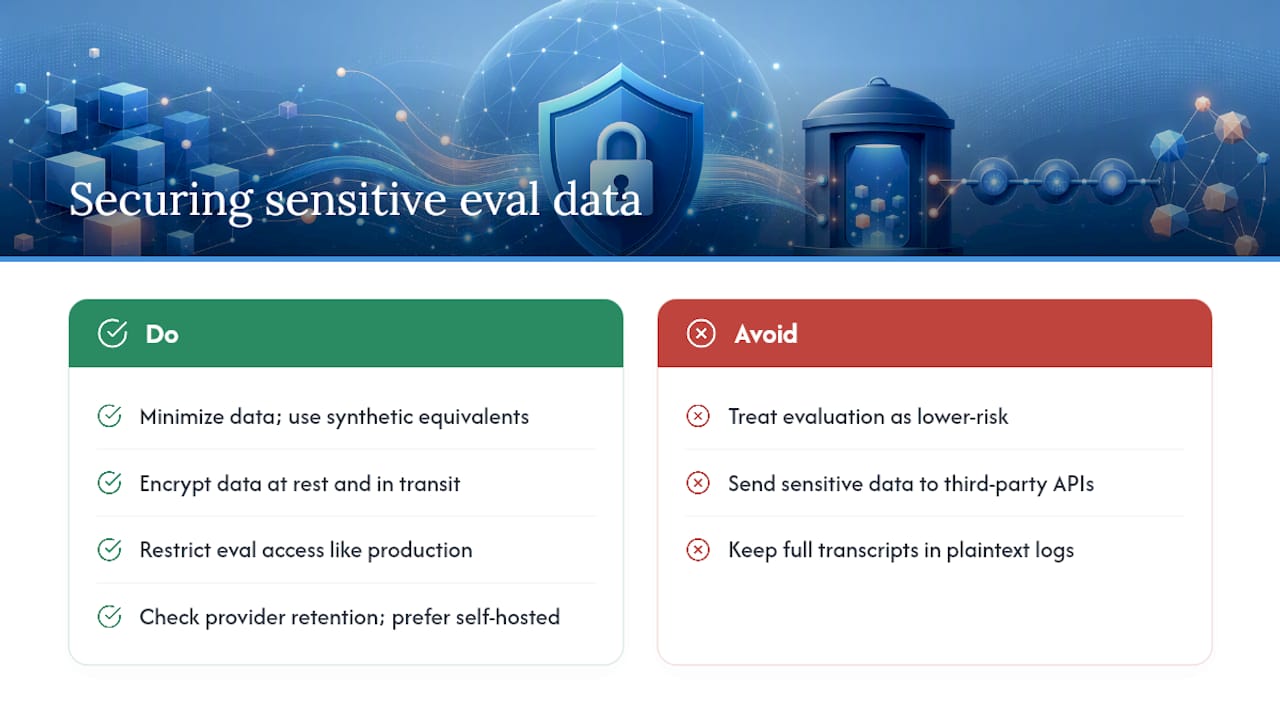
Evaluation datasets often contain exactly the kind of data you don't want leaking: customer support transcripts, medical notes used to test a clinical assistant, financial records for a fraud-detection model. Treating an eval run as lower-risk than a production request is a mistake that shows up in audit findings, not benchmarks.

Start with data minimization. If a task doesn't need a real customer name or account number to test the behavior you care about, replace it with a synthetic equivalent before it ever enters the harness. Where real data is unavoidable, encrypt it at rest and in transit, and restrict access to the evaluation environment the same way you'd restrict access to production data, not a looser standard because "it's just testing."

Provider choice matters here too. Sending sensitive evaluation data to a third-party model API means that data leaves your infrastructure, subject to that provider's retention and training-use policies. Check whether your provider offers a no-retention or zero-data-retention agreement before running sensitive tasks through it, and prefer self-hosted or enterprise-tier endpoints when the data warrants it.

Logging is the quiet risk most teams miss. Full transcripts captured for debugging agentic traces can sit in plaintext logs indefinitely, well past the point anyone remembers they're sensitive. Apply the same retention and redaction policies to eval logs that you apply to production logs, and scrub or hash personally identifiable fields before they hit a dashboard that other teams can see.

Keeping Your Evaluation Suite Current Over Time​

An evaluation harness that worked perfectly a year ago can be quietly lying to you today. Datasets go stale, models get better at gaming known benchmarks, and metrics that once distinguished good from bad models start clustering everyone near the ceiling.

Public benchmark saturation is the clearest sign. When most frontier models score above 90% on a benchmark, it's stopped discriminating between them, and you need a harder task or a fresh dataset slice to see real differences. Schedule a periodic review, quarterly is a reasonable cadence for active projects, to check whether your current suite still separates strong runs from weak ones.

Contamination creeps in from an unexpected direction: your own historical outputs. If a model's past responses to your eval set end up in a future training corpus (yours or a provider's), that task stops measuring generalization and starts measuring memorization. Rotating in fresh examples, or holding back a portion of your dataset from any published reporting, protects against this.

Metric relevance shifts too. A metric scorecard built around a model's early weaknesses can become irrelevant once those weaknesses get fixed elsewhere, while missing whatever new failure mode has emerged. Revisit your scorecard whenever you make a material change to the system under test, not just on a fixed schedule. Version your dataset and metric changes the same way you version prompts and tasks, so you can tell whether a score shift came from the model or from your own eval suite changing underneath it.

Author Perspective: Practical Tradeoffs and Prioritization​

Most teams get the build order backwards. They chase metric breadth first, wiring up five scoring methods before they've built a runner that reliably reproduces last week's results. Start with reproducibility and a minimal runner. One dataset, one metric, fully versioned, rerunnable on demand. Expand the metric suite only once that foundation holds.

LLM-as-a-Judge is the right call for scale, but treating it as a finished tool rather than a calibrated instrument is where teams get burned. Validate against human labels regularly, not once at launch. Judges drift, model updates shift their behavior, and a rubric that worked in January can quietly degrade by summer.

The unglamorous habit that separates durable harnesses from disposable ones: document every task and prompt as a versioned artifact from the first day, not after the third time someone asks "why did this score change?" The tension between owning your evaluation pipeline and depending entirely on a third-party model is worth sitting with here. A harness you fully control and version is part of how you keep ownership of your product's quality, rather than outsourcing that judgment entirely to whichever provider you're calling.

— Kevin

Put These Patterns to Work With MLflow​

Building the four components described here, dataset loaders, a runner, provider adapters, and scorers, from scratch is a real engineering project. A platform can provide a working foundation for all four components without starting from an empty repository, which matters most in the early weeks when reproducibility habits get set for good or get skipped under deadline pressure.

The platform's AI observability tooling handles the tracing layer described in the implementation patterns section, capturing agentic reasoning and tool calls rather than just final outputs. Its LLM-as-a-Judge support covers the scorer layer, including the calibration workflow that keeps a judge model honest against human review over time. Prompt versioning can help close the reproducibility gap that causes many "we can't reproduce last quarter's numbers" incidents.

If you're evaluating whether to build a harness from scratch or extend an existing platform, start with Mlflow's GenAI and agent engineering documentation for a quickstart and a sample repository you can run against your own models today.

Sources​

• A Practical Guide for Evaluating LLMs and LLM-Reliant Systems (2025)
• Evaluation metrics | Microsoft Learn

For production LLM apps, adopt a self-hostable observability stack that combines span-level tracing, automated evaluation through LLM-as-a-judge, and prompt management with version control. Open source LLM observability built on these three pillars catches quality regressions before users do. An open-source option built on this exact model is available, and OpenTelemetry gives you the standards-based instrumentation layer to connect it to whatever you already run.

---

TL;DR:

• Most teams fail to connect observability metrics directly to quality evaluation, risking blind spots in hallucination and factual accuracy.
• Focus on capturing granular trace data, including retrieval, tool calls, and multi-turn conversations, for effective debugging and analysis.
• Automated evaluation pipelines with LLM-as-a-judge are essential to scale quality checks versus manual review bottlenecks.
• Using standards like OpenTelemetry ensures trace portability across different backends, preventing vendor lock-in.
• Prioritize testing observability UI during simulated incidents to ensure quick identification of issues under real conditions.

---

Table of Contents​

• What Is LLM Observability, and Why Does It Matter for Production Apps?
• Key Features to Look for in an Open Source LLM Observability Stack
• How to Instrument an LLM Application: A Practical Implementation Checklist
• How MLflow Approaches LLM Observability
• Best Practices for Observability-Driven LLM Development
• What Actually Separates Teams That Succeed With Open Source Observability
• Get Started With MLflow for Open Source LLM Observability

What Is LLM Observability, and Why Does It Matter for Production Apps?​

Traditional application performance monitoring (APM) tracks whether a service is up, how fast it responds, and where it throws errors. That tells you almost nothing about whether your LLM app is actually working. A chatbot can return a 200 status code in 400 milliseconds, and still hallucinate a refund policy that doesn't exist. LLM observability exists to catch that gap between "the system ran" and "the system was right."

The vocabulary here matters because it maps to how you'll structure your data. A trace is the full record of one request through your system, from the initial prompt to the final response. A span is one step inside that trace, such as a retrieval call, a tool invocation, or a single model completion. Group related traces into sessions when you're tracking a multi-turn conversation, and build evaluation datasets from real production traffic so your quality checks reflect what users actually ask.

Four signal categories dominate any serious LLM monitoring setup:

• Cost: token spend per request, per feature, and per user segment.
• Latency: time to first token and total completion time, especially for streaming responses.
• Token usage: input/output ratios that reveal prompt bloat or inefficient context windows.
• Quality and hallucination rate: how often outputs drift from grounded, factual, or policy-compliant answers.

Standards-based instrumentation matters more than it sounds. Building a proprietary tracing format locks you into one vendor's dashboards forever. OpenTelemetry gives LLM apps the same portability that traditional infrastructure monitoring has had for years, letting you route trace data anywhere without re-instrumenting your code every time you change backends.

Key Features to Look for in an Open Source LLM Observability Stack​

Not every open source model tracking project covers the same ground. Before you commit engineering time to any stack, run it against this checklist.

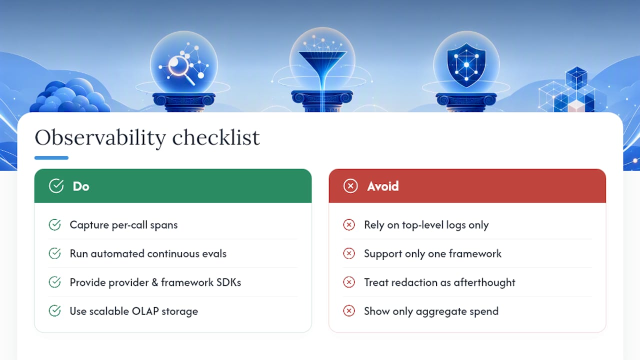
Tracing granularity. You need per-call spans, not just top-level request logs. That means capturing retrieval spans (what did the vector database actually return), tool-call spans (which function did the agent invoke and with what arguments), and session-level grouping so you can replay an entire multi-turn conversation instead of staring at disconnected fragments.

Automated evaluation pipelines. Manual review doesn't scale past a demo. Look for built-in support for LLM-as-a-judge, where a separate model scores outputs against a rubric for factuality, tone, or task completion. The strongest projects let you run these evals continuously against production samples, not just at release time, turning evaluation into a quality gate rather than a postmortem tool.

Provider and framework integrations. Confirm SDK coverage for the frameworks you actually use, whether that's LangChain, a custom agent loop, or direct API calls to a model provider. A tool that only supports one framework becomes dead weight the moment your architecture changes.

Storage and scale architecture. Trace volume grows fast, and a chatty agent can generate dozens of spans per user turn. Many open-source observability projects lean on OLAP-style backends like ClickHouse to handle high-throughput ingestion while keeping analytical queries fast. Confirm the project's storage layer can survive your actual traffic, not just a demo dataset.

Security and redaction. Prompts and outputs routinely contain names, emails, account numbers, and other data you don't want sitting in plaintext logs. Redaction and PII scanning should be a first-class feature, not an afterthought you bolt on later. Several open-source projects build string redaction and telemetry opt-out directly into their logging layer, which is the right place for it.

Cost observability. Token accounting needs to break down by model, endpoint, and business unit, not just show a single aggregate spend number. Without that granularity, you can't tell whether a cost spike came from a runaway retry loop or a genuinely higher-traffic day.

Developer ergonomics. A trace viewer that takes five clicks to find a failed span will get ignored during an incident. Look for a UI that supports fast filtering, side-by-side prompt comparison, and a playground where you can replay a captured trace with a modified prompt.

Pro Tip: Test any observability tool's UI during a simulated incident, not during a calm demo. Load fifty traces, inject a deliberately bad one, and time how long it takes you to find it. That number tells you more than any feature list.

How to Instrument an LLM Application: A Practical Implementation Checklist​

Instrumentation projects stall when teams try to capture everything on day one. Work through this in order instead.

1. Decide what to capture first. At minimum: the span structure (call boundaries), the exact prompt sent to the model, model parameters (temperature, max tokens, model version), retrieval context if you use RAG, and any human or automated annotations added after the fact. Skipping model parameters is the single most common gap teams regret, because you can't debug a regression if you don't know which model version produced it.

2. Choose your ingestion path. You have three realistic options: a vendor SDK embedded directly in your code, an OpenTelemetry adapter that instruments model calls and vector database activity automatically, or a gateway proxy that sits between your app and the model provider. The OpenTelemetry path is worth defaulting to if you already run Datadog, Honeycomb, or a similar backend, since it exports standard trace data your existing dashboards can already read.

3. Set storage and retention rules. Keep hot, full-fidelity traces for a shorter window (a week or two is common) and roll aggregated metrics into longer-term storage. Sampling matters here: capture 100% of error traces and a statistically meaningful sample of successful ones, rather than trying to keep everything forever at full detail.

4. Automate evaluation and wire it into CI. Curate a dataset of representative prompts, define your LLM-as-a-judge rubric, and run it against every pull request that touches prompt templates or model configuration. This is what separates observability-driven development from occasional manual spot-checks.

5. Set SLOs and alerts. Define acceptable thresholds for latency (say, time-to-first-token under a target you've validated with users) and quality (hallucination rate under a threshold measured by your eval suite). Alert on both. Test every alert path in staging before you trust it in production.

6. Run through a privacy checklist. Confirm redaction rules for PII before any prompt data hits persistent storage, lock down access controls to trace data by role, and give users or internal teams a documented telemetry opt-out where your data governance policy requires one.

A pattern worth calling out explicitly: for agentic workflows, capture both the agent's step metadata (tool calls, the action chosen) and the underlying LLM span together. Reconstructing a reasoning chain after the fact is nearly impossible if you only logged the final output and none of the intermediate decisions.

How MLflow Approaches LLM Observability​

Some platforms are built around the same three pillars this checklist walks through: tracing, evaluation, and prompt governance, applied specifically to agentic and GenAI workloads rather than bolted onto a generic ML monitoring tool.

Deep tracing of agentic reasoning is the core piece. MLflow captures each step an agent takes, including tool calls and intermediate decisions, alongside the LLM spans themselves, which directly satisfies the "capture agent metadata plus the LLM span together" pattern that makes agent debugging tractable instead of guesswork.

For evaluation, MLflow's LLM-as-a-Judge framework automates the scoring step that used to require a human reviewer reading through transcripts one at a time. You define the rubric, point it at a dataset, and get consistent scoring you can track release over release. A deeper technical walkthrough of how the judge model evaluates outputs is worth reading if you're designing your own rubric from scratch.

On the governance side, centralized AI Gateways handle prompt management and versioning across providers, so switching a model or rolling back a prompt template doesn't mean hunting through scattered config files. That maps directly to the "choose your ingestion path" and "prompt version control" checklist items above.

• Tracing: agentic reasoning traces plus standard LLM spans, unified in one system.
• Evaluation: automated LLM-as-a-Judge pipelines you can run in CI.
• Governance: AI Gateway for cross-provider prompt management and versioning.
• Deployment: self-hosted by default, with enterprise support options for teams that need bespoke integration or compliance guarantees.

Pro Tip: If you're migrating from ad hoc logging to structured observability, start by instrumenting just your highest-traffic endpoint with MLflow's tracing before rolling it out everywhere. You'll catch integration issues on one code path instead of ten.

Teams that need more than the self-hosted core can browse practical implementation guides covering SDK integration and deployment patterns in more depth than any single article can cover.

Best Practices for Observability-Driven LLM Development​

The teams that get real value from open source AI observability tend to run the same loop repeatedly: capture, evaluate, label, experiment, release. Skipping any single step in that cadence is usually where quality problems sneak back in.

Capture every production request by default, then evaluate a sample continuously rather than only after a user complains. Label the outputs your eval flags as questionable, feeding a growing dataset of edge cases back into your test suite. Experiment against that dataset before you ship a prompt change, and only then release, watching your quality dashboards closely for the first few hours.

Signal prioritization matters just as much as the cadence. Quality alerts (hallucination rate crossing a threshold, context loss in long conversations) should page someone faster than a pure latency blip, because a slow answer frustrates one user while a wrong answer can damage trust at scale. Infrastructure alerts, like queue depth or provider rate limits, belong on a slower, batched notification channel unless they're severe enough to cause outright failures.

Retention and sampling decisions come down to a straightforward tradeoff:

Approach	Fidelity	Cost	Best for
Full trace retention, no sampling	Highest	Highest	Low-traffic apps, early-stage debugging
100% error capture, sampled success	High for failures	Moderate	Most production apps past initial launch
Aggregated metrics only, short-lived traces	Lowest	Lowest	High-volume apps with mature eval pipelines

Team process closes the loop. Annotation work needs a clear owner, whether that's a rotating on-call engineer or a dedicated quality reviewer, and incident response for a quality regression should follow the same discipline as an infrastructure outage: a named owner, a documented root cause, and a dataset update so the same failure gets caught automatically next time.

What Actually Separates Teams That Succeed With Open Source Observability​

Most teams get the tracing part right on the first try and the evaluation part wrong. It's the easier half technically, so it gets built first, and then teams stop, satisfied they can now "see" what their LLM is doing. Seeing isn't the same as judging. A trace viewer full of colorful spans feels like progress, but if nothing is scoring those traces against a rubric, you've built a very expensive log viewer.

The self-hosted versus hybrid question comes up constantly, and the honest answer depends on your compliance posture more than your engineering preference. Full self-hosting gives you complete control over where prompt data lives, which matters enormously if you're handling regulated data or operating under contractual data residency requirements. A hybrid approach, where you self-host tracing but lean on a managed eval service, can get you moving faster, but it means sending production prompts to a third party. Read your data governance policy before you pick, not after.

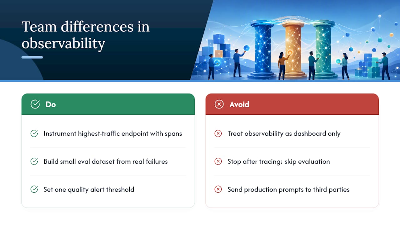
The biggest overlooked pitfall isn't technical at all. It's treating observability as a monitoring dashboard instead of a development practice. The teams that actually improve their models over time run evaluation as part of their pull request process, the same way they'd run unit tests. The teams that struggle bolt observability on after an incident, look at it for a week, then forget it exists until the next fire.

Three things worth doing this week: instrument your single highest-traffic endpoint with span-level tracing if you haven't already, build one small evaluation dataset from real production failures instead of synthetic examples, and set one quality alert threshold even if it's a rough guess. A rough alert beats no alert.

— Kevin

Get Started With MLflow for Open Source LLM Observability​

MLflow gives you a working implementation of everything covered above, not a partial toolkit you have to stitch together with three other projects. Tracing, automated evaluation, and prompt governance live in one open-source platform instead of scattered across a homegrown logging layer, a separate eval script, and a spreadsheet tracking prompt versions.

The AI Observability product page walks through the tracing and monitoring features directly, and the Agent & LLM Engineering platform covers how observability connects to orchestration and deployment for teams running production agents. Both are self-hostable from day one, with enterprise support available for teams that need compliance guarantees or bespoke integration work beyond what the open-source core covers.

If you're evaluating tools this quarter, the fastest path is to instrument one endpoint and run your first automated evaluation before committing further engineering time. Start with the observability overview and see how quickly you can get a real trace into the system.

Recommended​

• One post tagged with "how to enhance LLM observability"
• Setting Up LLM Observability Pipelines in 2026
• One post tagged with "how to monitor LLM outputs"
• One post tagged with "LLM data flow monitoring"

Deploying a large language model to production and assuming your existing monitoring stack will catch failures is one of the most common and costly mistakes AI ops teams make today. Understanding what is LLM observability, and why it differs fundamentally from traditional system monitoring, is now a core competency for any team running LLMs at scale. Your infrastructure dashboards can show green across the board while your model is confidently generating hallucinated facts, violating content policies, or drifting away from your intended use case. This guide breaks down what LLM observability actually covers, how to implement it, and why getting it right is non-negotiable for enterprise deployments.

Table of Contents​

• What is LLM observability and why does it matter?
• Core components of LLM observability: tracing, metrics, and evaluations
• Why traditional monitoring falls short for large language models
• Implementing LLM observability in enterprise environments
• Why traditional AI monitoring approaches won’t cut it for LLMs
• Streamline your LLM observability with MLflow AI platform
• Frequently asked questions

Key Takeaways​

Point	Details
LLM outputs require semantic monitoring	LLM observability tracks output quality and safety beyond traditional system health metrics.
Tracing links failures to root causes	Combining trace data with quality evaluations accelerates debugging and reduces investigation time.
Prompt tracking is crucial	Monitoring prompt templates and versions helps correlate changes to performance and output quality.
LLM observability improves reliability	Continuous monitoring of LLMs enables early anomaly detection and helps maintain alignment with business goals.
MLflow supports end-to-end observability	MLflow provides SDKs and tools for instrumentation, tracing, evaluation, and cost monitoring in production LLMs.

What is LLM observability and why does it matter?​

LLM observability is the practice of continuously monitoring, tracing, and evaluating the behavior of large language models across the full application lifecycle. It extends far beyond infrastructure metrics. As LaunchDarkly documents, LLM observability analyzes how models behave across development, testing, and production by tracking inputs, outputs, latency, quality, safety, and cost.

The distinction from traditional observability is significant. With a conventional API or database, a successful response means the system did what it was supposed to do. With an LLM, a 200 OK response only tells you the model returned something. Whether that something is accurate, relevant, safe, or aligned with your business goals is an entirely separate question, and one that standard monitoring tools cannot answer.

The AI observability overview from MLflow captures this well: observability for AI systems must account for the semantic dimension of outputs, not just the operational one. For enterprise teams, this means building monitoring pipelines that cover:

• Input tracking: Logging every prompt, including template versions and injected variables
• Output evaluation: Assessing responses for correctness, relevance, toxicity, and hallucinations
• Latency and throughput: Measuring end-to-end response times and throughput under load
• Token usage and cost: Tracking per-request token consumption to manage spend
• Safety and alignment checks: Detecting policy violations, off-topic responses, and prompt injections
• Drift detection: Identifying when model behavior shifts over time, even without a code change

Each of these dimensions addresses a failure mode that traditional monitoring simply cannot see. That is the core argument for LLM observability as a distinct practice.

Core components of LLM observability: tracing, metrics, and evaluations​

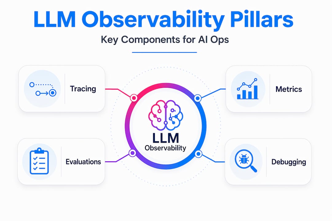
Now that we’ve introduced the need for LLM observability, let’s look at the specific technical pillars that make this practice work in production. There are three primary components: tracing, metrics, and evaluations. Together, they give your team a complete picture of system health and output integrity.

Tracing maps the full lifecycle of a request through your LLM application. This includes the initial prompt, any retrieval steps in a RAG pipeline, calls to external tools or APIs, sub-agent invocations, and the final model response. LLM tracing techniques are essential for root cause analysis because they let you pinpoint exactly where in a complex workflow something went wrong, rather than hunting through disconnected logs.

Metrics are the quantitative signals your team needs to track continuously. As Elastic’s LLM observability documentation outlines, LLM observability includes tracing each request through the stack, capturing token usage and cost, tracking latency and errors, and running quality and safety evaluations on outputs. On the instrumentation side, Datadog’s approach supports capturing prompts and completions, token usage, latency, error info, and model parameters.

Evaluations are what truly separate LLM observability from everything that came before. These are automated or human-in-the-loop assessments of whether model outputs meet defined quality criteria. Evaluations for LLMs typically include:

1. Relevance scoring: Does the response address what the user actually asked?
2. Faithfulness checks: In RAG systems, is the answer grounded in the retrieved context?
3. Hallucination detection: Did the model fabricate facts, names, or citations?
4. Toxicity and safety: Does the response contain harmful, biased, or policy-violating content?
5. Task-specific rubrics: Custom criteria aligned to your application’s business requirements

Here is a quick reference for the three pillars and what each captures:

Component	What it captures	Why it matters
Tracing	Request flow, spans, tool calls, sub-agents	Root cause analysis in complex workflows
Metrics	Token count, cost, latency, error rate	Operational health and spend management
Evaluations	Quality, relevance, safety, hallucinations	Output integrity and business alignment

Pro Tip: Wire your evaluations directly to individual traces, not just aggregate reports. When an evaluation flags a low-quality response, you want to jump straight to the exact prompt, context, and model parameters that produced it. Aggregate scoring alone tells you there is a problem. Trace-linked evaluation tells you why.

Why traditional monitoring falls short for large language models​

Understanding these components helps clarify why traditional monitoring misses key LLM failure modes. The gap is not a matter of degree. It is structural.

Traditional monitoring was built around a simple contract: if the system returns a valid response within an acceptable time, the request succeeded. That contract holds for deterministic systems. An API that returns the wrong JSON is a bug you can catch. A database query that returns stale data triggers an alert. The failure is visible at the infrastructure layer.

LLMs break this contract entirely. As Swept AI’s observability guide notes, an LLM can have sub-second latency and 200 OK status yet produce fabricated, harmful, or off-topic content undetectable by traditional monitoring. Your uptime monitor sees a healthy system. Your user sees a confidently wrong answer.

“Infrastructure metrics alone miss hallucinations and incorrect outputs even when requests technically succeed.” — Swept AI LLM Observability Guide

The failure modes unique to LLMs include:

• Hallucinations: The model generates plausible-sounding but factually incorrect information
• Topic drift: Responses gradually shift away from intended use cases without any code change
• Prompt injection: Malicious inputs manipulate the model into ignoring system instructions
• Refusal failures: The model refuses valid requests due to overly aggressive safety tuning
• Bias amplification: Outputs reflect or amplify demographic or ideological biases present in training data

None of these show up in your existing production observability challenges tooling unless you build explicitly for them. A customer-facing LLM that starts hallucinating product specifications will not trigger a single alert in a traditional monitoring stack. The only signal you get is a surge in support tickets, or worse, a public incident.

Implementing LLM observability in enterprise environments​

With these challenges in mind, let’s explore how enterprise teams actually build practical observability into their LLM deployments. The good news is that the implementation path is well-defined, even if the tooling is still maturing.

1. Instrument your application with an observability SDK. The fastest path to tracing and metric collection is integrating an SDK that auto-instruments your LLM calls. Getting started with MLflow tracing requires minimal code changes and immediately begins capturing spans, token counts, and latency for every request.
2. Treat prompts as versioned artifacts. Prompt templates are the primary lever teams use to change model behavior, but they are often managed as strings in a config file. Treating prompts as first-class observables helps correlate prompt changes with latency, cost, and evaluation metrics. When a quality regression appears, you can immediately check whether a prompt version change preceded it.
3. Link evaluations to traces. Run automated evaluations on every response, or a statistically significant sample, and attach the results to the originating trace. Datadog reports a roughly 20x reduction in debugging time by correlating evaluator failures with trace-level context. That is the difference between knowing a problem exists and knowing exactly where to fix it.
4. Set up cost and safety dashboards with proactive alerts. Token costs can spike unexpectedly when users find creative ways to send long prompts. Safety violations can cluster around specific input patterns. Dashboards that surface these signals in real time, with alerts that fire before costs or risks escalate, are essential for production operations.

Here is a practical breakdown of what to instrument at each stage of your deployment:

Deployment stage	Key observability actions	Primary benefit
Development	Trace all LLM calls, log prompt versions	Catch regressions before they ship
Staging	Run LLM-as-a-Judge evaluations on test sets	Validate quality against baselines
Production	Monitor cost, latency, safety, and drift	Detect failures before users report them
Post-incident	Replay traces with updated prompts	Confirm fixes without re-deploying

Pro Tip: Do not wait for user complaints to discover quality regressions. Set up automated evaluation runs on a rolling sample of production traffic and alert on any statistically significant drop in your quality scores. This is the LLM equivalent of synthetic monitoring, and it catches problems hours or days before they surface in user feedback.

Why traditional AI monitoring approaches won’t cut it for LLMs​

Here is the uncomfortable truth we have observed working with enterprise AI teams: most organizations treat LLM observability as something they will add later, once the model is “stable.” That framing misunderstands what stability means for probabilistic systems.

LLM outputs are probabilistic and drift over time, so teams must observe both system performance and model behavior to catch anomalies. A model does not need a code change to start behaving differently. A provider model update, a shift in user input distribution, or a subtle change in retrieved context can all alter output quality without touching a single line of your application code. If you are not observing outputs continuously, you will not know until the damage is done.

We also see teams conflate evaluation with testing. Running an eval suite before deployment is necessary but not sufficient. Production inputs are messier, more varied, and more adversarial than any test set. The LLM evaluation perspective we advocate is that evaluation is a continuous process, not a gate. It belongs in your monitoring pipeline, not just your CI/CD workflow.

The rise of autonomous LLM agents makes this even more critical. When a model is not just answering questions but taking actions, calling APIs, and making decisions in multi-step workflows, an undetected failure does not just produce a bad response. It can trigger a cascade of incorrect actions that are difficult to reverse. Observability at the agent level, tracing every reasoning step and tool call, is the only way to maintain meaningful oversight of these systems.

Output correctness is a separate dimension from system health. Treating them as the same problem is how teams end up with production LLMs that are technically healthy and operationally broken.

Streamline your LLM observability with MLflow AI platform​

If you are building or scaling LLM applications in production, the gap between what your current monitoring covers and what LLM observability requires is real and consequential. MLflow was built to close that gap.

MLflow LLM observability gives your team end-to-end instrumentation with minimal code changes, capturing traces, token metrics, and evaluation results in a unified platform. You can correlate prompt versions with quality scores, drill into individual traces when evaluations flag failures, and monitor cost and safety signals from a single dashboard. For teams running complex agentic workflows, MLflow AI observability provides deep tracing of multi-step reasoning chains and sub-agent interactions. MLflow LLM tracing integrates with the frameworks your team already uses, so you get production-grade visibility without rebuilding your stack.

Frequently asked questions​

What is the difference between LLM observability and traditional monitoring?​

LLM observability includes monitoring of model outputs for quality, safety, and relevance, whereas traditional monitoring focuses mainly on system health metrics like uptime and latency. As LaunchDarkly’s guide notes, LLM observability extends traditional monitoring by tracking semantic output evaluations in addition to infrastructure metrics.

Why can an LLM response be a failure even if the latency and error rates are low?​

Because LLMs generate probabilistic outputs, a response can be incorrect, hallucinatory, or unsafe even if the system returns quickly without errors. LLMs can produce fabricated or harmful content despite successful system performance signals like sub-second latency and HTTP 200 status.

How does tracing help reduce debugging time for LLM applications?​

Tracing correlates evaluation failures with exact request and workflow details, enabling faster identification of issues within complex LLM workflows. Datadog reports 20x faster debugging by linking evaluator failures to trace-level context for LLM agents.

What are key metrics to monitor with LLM observability?​

Important metrics include token usage and cost, latency, error rates, model parameters, and quality evaluations such as hallucination detection and topic relevance. Datadog’s instrumentation captures prompts, completions, token usage, costs, latency, errors, and model parameters including temperature and max tokens.

Can LLM observability detect prompt injection attacks or content policy violations?​

Yes, observability tools can monitor prompts and responses for harmful content and detect injection attempts, helping enforce safety guardrails. Elastic’s LLM observability monitors for prompt injection attacks and tracks policy-based interventions with built-in guardrails support.

Recommended​

• AI Observability for LLMs & Agents | MLflow AI Platform
• LLM Tracing & AI Tracing for Agents | MLflow AI Platform
• AI Monitoring for LLMs & Agents | MLflow AI Platform
• Agent & LLM Evaluation | MLflow AI Platform