2 posts tagged with "monitoring machine learning models"

Alerts are the action boundary of ML monitoring: they convert observed model and data problems into immediate, documented responses. Passive monitoring tells you what is happening; alerts tell your team that something requires a response right now. The distinction matters more than most teams realize when they first wire up a monitoring stack.

The role of alerts in ML monitoring breaks down into three core functions:

• Detect urgent change — fire when a signal crosses a threshold or a statistical test flags a distribution shift that exceeds your business tolerance.
• Assign ownership and route response — page the right on-call engineer, open a ticket, or trigger an automated mitigation, depending on severity.
• Point to diagnostics and runbooks — every alert should carry a link to the affected model run or artifact and a documented investigation path.

Not every signal belongs in an alert. A sudden accuracy collapse on your primary revenue model warrants a P1 page. Slow seasonal drift in a secondary feature warrants a dashboard annotation and a weekly review, not a 2 AM wake-up. Getting that boundary right is what separates a team with a healthy on-call rotation from one drowning in noise.

Google SRE practices formalize this through SLO/error-budget framing: rather than alerting on raw metric values, you alert when error-budget burn rate exceeds a threshold that signals the SLO will be exhausted before the next review window. Mlflow extends this model into the ML layer by linking alert context directly to run IDs and model registry entries, so responders can pull the exact training artifacts and evaluation logs the moment an alert fires.

---

Key Takeaways​

Alerts are the operational contract between your monitoring system and your on-call team: they only work when every alert is owned, linked to a runbook, and validated before it reaches a pager.

Point	Details
Alerts vs. monitoring	Alerts demand an immediate, documented response; monitoring supports investigation and trend analysis.
Signal prioritization	Start with business-proxy and output KPIs; add input feature monitors only where they predict output degradation.
Threshold design	Compute baselines at deploy time, use PSI/KS comparisons, and apply debounce windows and inhibition rules to cut noise.
Runbooks and ownership	Every alert must carry a runbook URL, a named owner, and an Mlflow run ID for rapid root-cause analysis.
Mlflow integration	Attaching Mlflow run IDs and model registry versions to alert payloads shortens RCA and supports reproducible incident response.

---

Table of Contents​

• What's the difference between monitoring and alerting in ML?
• What signals and metrics should feed your ML alerts?
• Which alert detector type fits your use case?
• How do you design thresholds that don't cause alert fatigue?
• How should alert routing, ownership, and escalation work in practice?
• How do you build response playbooks that actually get used?
• What tooling and integrations does a production ML alerting stack need?
• What can teams learn from LinkedIn AlerTiger's production ML alerting?
• How do you test and validate alerts before they hit production?
• What are the most common ML alerting anti-patterns?
• A practical perspective on running ML alerting in production
• Mlflow gives you traceable alerts from day one
• Sources

What's the difference between monitoring and alerting in ML?​

Monitoring and alerting are complementary but operationally distinct. Monitoring is the continuous collection, storage, and visualization of signals: dashboards, trend lines, anomaly scores, and distribution plots that data scientists use to understand model behavior over time. Alerting is the narrow, urgent layer on top: a predefined rule that fires when a signal crosses a threshold and demands an explicit, time-bounded response.

The primary consumer of monitoring is a data scientist or ML engineer doing investigation and trend analysis. The primary consumer of an alert is whoever is on-call right now, and they need to know exactly what to do in the next 15 minutes. Nubank's engineering team puts it plainly: alerts are for urgent problems that require immediate, predefined responses, while monitoring supports deeper investigation. Conflating the two is the fastest path to alert fatigue.

Signal	Time horizon	Primary consumer	Monitoring or alerting?
Prediction latency p99	Real-time	On-call engineer	Alerting (P1 if SLO breach)
Model accuracy (rolling 24h)	Daily	Data scientist	Both: dashboard + P1 alert on collapse
PSI on key feature	Weekly	ML engineer	Monitoring (warning alert at PSI > 0.2)
Prediction entropy drift	Hourly	On-call / ML engineer	Alerting (P2 if sustained)
Feature pipeline error rate	Real-time	On-call engineer	Alerting (P1 if > threshold)
Seasonal accuracy trend	Monthly	Data scientist	Monitoring only

Pro Tip: Every alert you create should include a direct link to the diagnostic dashboard for that model and the Mlflow run ID of the currently deployed version. A responder who has to hunt for context wastes minutes that compound into SLO violations.

---

What signals and metrics should feed your ML alerts?​

Start from business impact, not from raw input distributions. A practitioner's guide from the MLOps Community is explicit: teams that wire up alerts on every input feature change first produce mostly low-value noise. The right sequence is output KPIs first, then prediction distributions, then input features.

The core signal categories and their measurement methods:

• Model performance metrics: accuracy, AUC-ROC, F1, calibration error, top-k accuracy. Measure on labeled ground-truth windows; cadence depends on label latency.
• Prediction distribution / prediction drift: prediction entropy, confidence-coverage curves, output histogram shifts. Jensen-Shannon divergence (JSD) works well for comparing output distributions across time windows.
• Input/feature distributions: Population Stability Index (PSI) and Kolmogorov-Smirnov (KS) test for continuous features; chi-squared for categoricals. Baseline at deploy time and route PSI warnings (0.1–0.2) to low-noise channels; route critical events (PSI > 0.2) to pager.
• Latency and availability: p50/p95/p99 inference latency, error rate, timeout rate. These are infrastructure-adjacent and often the fastest signals to detect serving failures.
• Feature pipeline / data health: null rate, schema violations, out-of-range values, pipeline job failure. A broken feature pipeline can silently degrade model inputs before any model metric moves.
• Business-proxy metrics: conversion rate, revenue per prediction, click-through rate. These are the ultimate ground truth for model health and should anchor your P1 alert definitions.

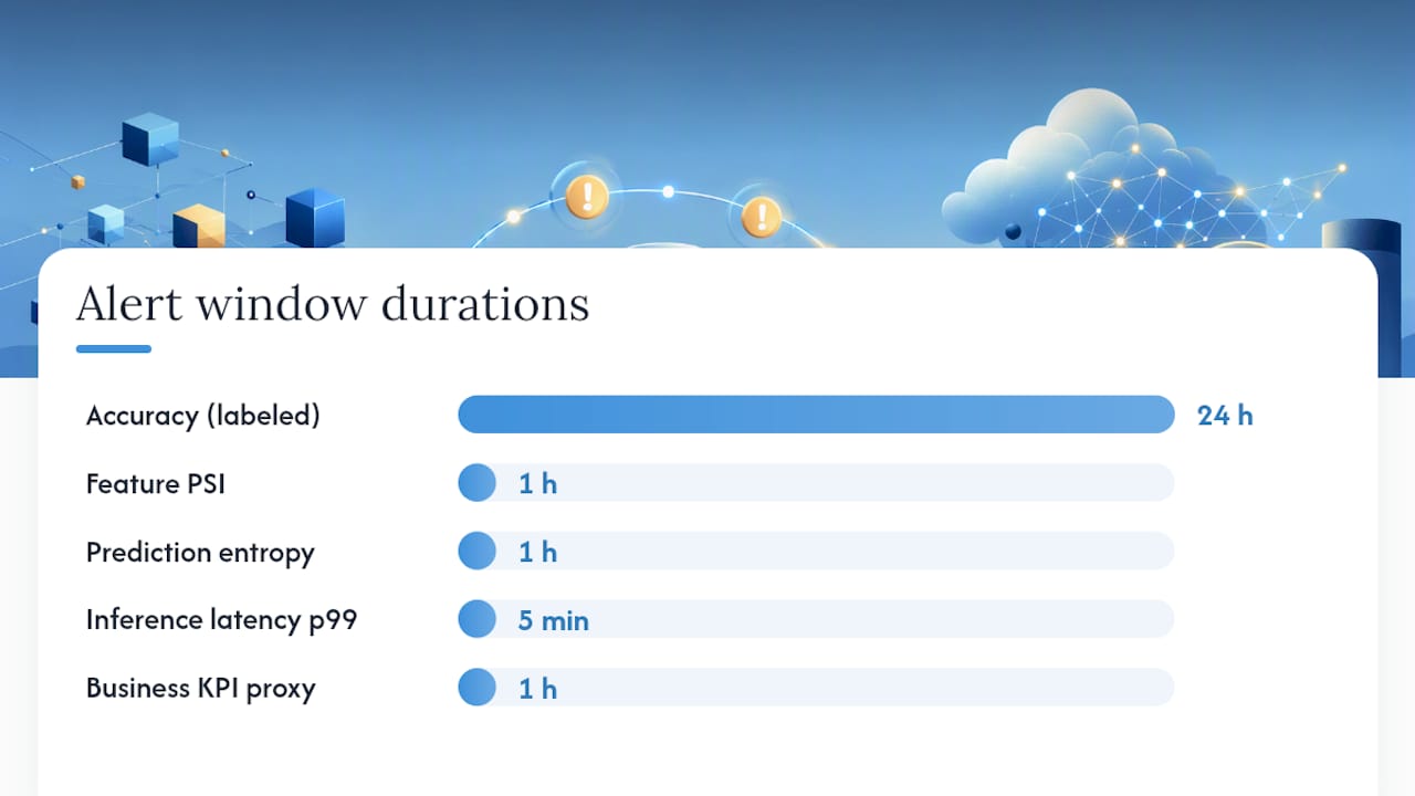
Signal	Statistic	Alert window	Suggested route
Accuracy (labeled)	Absolute drop vs baseline	24h rolling	P1 page if significant drop
Feature PSI	PSI score	1h rolling	P2 Slack if moderate drift; P1 page if significant drift
Prediction entropy	JSD vs reference	1h rolling	P2 Slack if sustained high value
Inference latency p99	Absolute ms vs SLO	5-min rolling	P1 page if latency exceeds SLO
Pipeline job failure	Binary (fail/pass)	Per run	P1 page immediately
Business KPI proxy	% change vs 7-day avg	1h rolling	P1 page if notable drop

---

Which alert detector type fits your use case?​

Three detector families cover most production ML alerting needs, and each has a distinct cost-benefit profile.

Threshold-based alerts​

Threshold detectors are deterministic: if metric X exceeds value Y for duration Z, fire. They are the lowest-maintenance option and the right default for well-understood infrastructure metrics like latency, error rates, and pipeline job failures. The failure mode is brittleness: a static threshold set at model launch drifts out of calibration as traffic patterns change, producing false positives in high-traffic periods and false negatives during low-traffic ones.

Statistical drift tests (KS, PSI, JSD)​

Statistical tests quantify how much a distribution has shifted from a reference window. The KS test measures the maximum distance between two empirical CDFs; PSI converts that into a binned stability score with interpretable thresholds (PSI < 0.1 is stable, 0.1–0.2 is moderate drift, > 0.2 is significant). JSD is symmetric and bounded, making it useful for comparing prediction distributions. The calibration challenge is choosing the right window size: too short and you get noise-driven alerts; too long and you miss fast-moving drift. Dynamic baselines and rate-of-change signals outperform static thresholds for these tests, especially when traffic volume varies.

ML-based anomaly detectors​

Learned detectors adapt to seasonality and complex multivariate patterns that rule-based systems miss. They handle feature interactions and temporal dependencies that PSI and KS cannot capture. The trade-off is explainability and maintenance: a neural anomaly detector that fires at 3 AM needs to tell the on-call engineer why it fired, not just that it did. Raw anomaly scores are not sufficient for an actionable page; post-processing and explainability steps are mandatory at production scale.

Detector type	Sensitivity	Explainability	Maintenance cost	Best for
Threshold	Low	High	Low	Latency, error rates, pipeline failures
Statistical (KS/PSI/JSD)	Medium	Medium	Medium	Feature/prediction drift, data quality
ML-based anomaly	High	Low (requires post-processing)	High	Complex multivariate, seasonal signals

KS test calibration note: A KS p-value below 0.05 indicates statistically significant distribution shift, but statistical significance is not the same as operational significance. With large sample sizes, trivial shifts become significant. Set alert thresholds on the KS statistic value itself (e.g., D > 0.1) rather than on p-value alone, and combine with a minimum sample size requirement.

PSI calibration note: PSI is sensitive to binning strategy. Use equal-frequency bins computed on the training reference distribution and keep bin count consistent across windows. A PSI of 0.1 on a 10-bin histogram is not equivalent to a PSI of 0.1 on a 20-bin histogram.

Pro Tip: Composite alerts — requiring two or more signals to co-occur before firing — are one of the most effective ways to cut false-positive rates. Require both a PSI > 0.15 on a key feature AND a prediction entropy increase before paging; either alone may be noise, but together they point to a real input shift affecting outputs. SLO/burn-rate alerting applies the same principle at the error-budget level.

---

How do you design thresholds that don't cause alert fatigue?​

Threshold design is where most teams lose the most time. The process below moves a detector from concept to production without burning out your on-call rotation.

1. Define the business impact first. What does a violation of this metric cost in revenue, user experience, or SLO budget? If you cannot answer that, you do not yet have enough information to set a threshold.
2. Choose the metric and measurement window. Match the window to the signal's natural cadence: latency alerts need 5-minute windows; accuracy alerts on labeled data may need 24-hour rolling windows because label latency is high.
3. Compute a baseline at deploy time. Capture the distribution of the metric during the first stable week post-deployment. This baseline is your reference for PSI and KS comparisons. Compute it at deploy time and version it alongside the model artifact.
4. Set warning and critical thresholds separately. Warning routes to Slack or a low-noise digest; critical routes to pager. The gap between them gives you a buffer to investigate before escalating.
5. Apply anti-noise controls. Use debounce windows (require the condition to hold for N consecutive evaluations before firing), moving-average comparisons instead of point-in-time values, and seasonality-aware baselines for metrics with weekly or daily cycles. Percentile thresholds (e.g., p95 latency) are more stable than absolute thresholds for high-variance metrics.
6. Define suppression and inhibition rules. If a pipeline job fails, suppress downstream model-accuracy alerts for that window — the accuracy drop is a symptom, not a separate incident. Inhibition rules prevent alert storms during known outages.
7. Convert business tolerance to SLO burn-rate triggers. If your SLO allows 0.1% error rate over 30 days, a burn rate of 14x means you will exhaust the budget in 2 days. Alert at a burn rate that gives you enough time to respond before the budget is gone.

Pro Tip: Treat your alert rules as code. Store them in version control, run them through CI on every change, and require a runbook link as a mandatory field before a rule can be merged. An alert without a runbook is a liability.

---

How should alert routing, ownership, and escalation work in practice?​

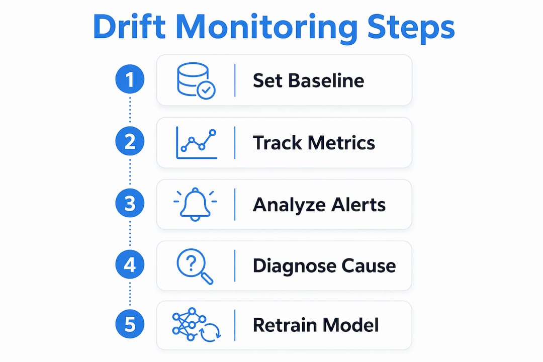
The alert lifecycle has seven steps, and skipping any of them creates operational debt: detect → notify → acknowledge → investigate → mitigate → post-mortem → tune.

Ownership is the most commonly skipped step. Every alert must have a named owner — a team or rotation, not just a channel. Unowned alerts get ignored. Alerts that lack documented investigation steps or links to a specific diagnostic dashboard become noise quickly; successful teams ensure every alert points to the affected model endpoint and the suspected features.

Standardize the structured fields every alert carries:

• model_id and model_version
• run_id (Mlflow run ID of the deployed artifact)
• feature_segment (which feature or segment triggered the alert)
• current_value vs baseline_value
• severity (P1/P2/P3)
• runbook_url
• diagnostic_dashboard_url

Escalation timelines should be explicit: if a P1 alert is not acknowledged within 5 minutes, escalate to the secondary on-call. If not mitigated within 30 minutes, escalate to the team lead. These timelines belong in the runbook, not in someone's memory.

Separate detection from notification architecturally. A layered pattern — observe → decide → act — lets you add deduplication, grouping, and inhibition rules between the detector and the pager. Production alerting systems that conflate detection and notification cannot suppress alert storms during cascading failures.

---

How do you build response playbooks that actually get used?​

A runbook that lives in a wiki page nobody can find during an incident is not a runbook. Every runbook needs these fields, and it needs to fit on one scrollable screen:

1. Alert name and severity
2. Preconditions — what must be true for this alert to fire (e.g., model is serving live traffic, feature pipeline ran successfully in the last hour)
3. Immediate checks — the first three queries or dashboard panels to open
4. Diagnostic queries — specific SQL, Python snippets, or Mlflow API calls to pull the relevant run metrics and feature distributions
5. Mitigation steps — ordered, numbered actions
6. Rollback criteria — when to cut traffic to the previous model version
7. Owner and escalation path
8. Communication steps — who to notify and what to say

Example playbook 1: P1 accuracy collapse​

• Check the feature pipeline status for the last 2 hours. If any job failed, the accuracy drop is likely a data issue, not a model issue.
• Pull the Mlflow run ID from the alert context. Compare current serving metrics against the registered baseline in the model registry.
• If accuracy is down more than 10% and the pipeline is healthy, cut traffic to the previous model version immediately using your serving layer's traffic-split control.
• Open an incident ticket with the run ID, current accuracy, and baseline accuracy attached.
• Notify the model owner and data engineering lead within 15 minutes.
• Trigger a retrain only after root cause is confirmed — retraining on corrupted data makes the problem worse.

Example playbook 2: Data drift on a key feature​

• Confirm the PSI value and the feature name from the alert context.
• Pull the feature distribution for the last 24 hours from your feature store and compare against the deploy-time baseline stored in Mlflow artifacts.
• Check upstream data sources for schema changes, pipeline delays, or source system anomalies.
• If drift is confirmed and upstream is clean, run the retrain decision checklist: Is labeled data available for the drift period? Is the drift likely to persist? Does the business KPI show impact?
• If all three are yes, open a retrain ticket. If not, add a monitoring annotation and schedule a review in 48 hours.

Do vs. don't:

• Do automate traffic cuts and rollbacks for P1 accuracy collapses when the rollback criteria are unambiguous.
• Don't automate retraining decisions — they require human judgment about data quality and business context.
• Do version runbooks alongside model registry entries in Mlflow so the runbook version matches the model version.
• Don't page humans for P3 signals — create a ticket and let the team triage it during business hours.

---

What tooling and integrations does a production ML alerting stack need?​

A production alerting stack has five layers, and each has distinct capability requirements.

Metrics collectors ingest model serving logs, feature pipeline outputs, and business KPI streams. They need low-latency ingestion and support for windowed aggregations.

Drift detectors run statistical tests (KS, PSI, JSD) or ML-based anomaly models against reference distributions. They need access to deploy-time baselines and should output structured drift scores, not just binary pass/fail.

Rule engine evaluates alert conditions, applies deduplication and grouping, and enforces inhibition rules. This is where composite alert logic lives.

Notification layer routes alerts to the right channel by severity: P1 to pager, P2 to Slack, P3 to email digest. It should support rich context attachments — Mlflow run IDs, artifact links, and runbook URLs — so responders have everything they need in the alert itself.

Incident management tracks acknowledgment, investigation notes, and resolution. Bidirectional integration with the rule engine lets resolved incidents automatically close alerts and feed tuning data back into threshold calibration.

Security and privacy considerations are often overlooked in alerting design. Alert payloads that include feature values may contain PII if the model operates on user data. Apply field-level masking before routing alerts to external notification channels. Runbook access should follow least-privilege: on-call engineers need read access to diagnostic dashboards and model artifacts, but not write access to production data stores. Audit logs for alert acknowledgment and escalation actions are a compliance requirement in regulated industries.

For monitoring pipeline setup and integration patterns, the architecture decision that matters most is keeping detection and notification separate. A monolithic system that detects and pages in the same step cannot implement inhibition rules or deduplication without significant rework.

---

What can teams learn from LinkedIn AlerTiger's production ML alerting?​

LinkedIn's AlerTiger is one of the most detailed public accounts of running ML-based anomaly detection at production scale across a large portfolio of AI features. The AlerTiger README describes a deep-learning time-series pipeline with four stages: statistics generation, anomaly detection, post-processing and explainability, and alert routing.

The design choices that made it work at scale:

• Normalization per feature: each feature's time series is normalized before entering the detector, so a single model can generalize across features with very different magnitudes and variance profiles.
• Seasonality adaptation: the model learns weekly and daily patterns, which prevents false positives during predictable traffic cycles that would trigger static-threshold alerts.
• Post-processing rules: raw anomaly scores from the neural detector are filtered through post-processing rules before any alert fires. This step is where most of the false-positive reduction happens.
• Explainability layer: the pipeline outputs not just an anomaly flag but a ranked list of contributing factors, so the on-call engineer knows which feature segment or time window drove the score.

The lessons that apply directly to teams adopting ML-based detectors:

• Feature and model lifespans are short. Your anomaly detector needs to handle features being added, removed, and retrained frequently without manual reconfiguration.
• Explainability is a product requirement, not a research nice-to-have. If your detector cannot tell the responder why it fired, it will not survive its first month in production.
• Post-processing is where you tune the precision-recall trade-off. Invest in it before you invest in a more complex detector architecture.
• Link every alert from your ML-based detector to the Mlflow run ID of the model that produced the flagged predictions. Without that link, RCA requires manual archaeology through logs.

---

How do you test and validate alerts before they hit production?​

Shipping an untested alert rule to a pager rotation is the fastest way to lose your team's trust in the alerting system. The validation process has four stages:

1. Historical backtesting. Replay labeled historical incidents through your alert rules and measure precision (what fraction of alerts corresponded to real incidents) and recall (what fraction of real incidents generated an alert). A rule with 40% precision is generating more noise than signal.
2. Synthetic incident injection. Inject known failure patterns — feature drift, latency spikes, accuracy drops — into a staging environment and verify that the correct alert fires within the expected window. Measure alert-to-incident lead time: how many minutes before the incident was confirmed did the alert fire?
3. Shadow alerting. Run the new alert rule in parallel with production for one to two weeks, logging all fires without routing them to pager. Review the shadow log daily to identify false positives and calibrate thresholds before enabling the pager integration. Backtesting and shadow-mode alerting are the two most effective pre-production validation steps.
4. Staged rollout. Enable the alert for a small on-call group first. Collect feedback on false-positive rate, time-to-ack, and runbook clarity before rolling out to the full rotation.

Track these metrics for every alert type in production:

• False-positive rate: alerts that fired but required no action
• Time-to-ack: median time from alert fire to acknowledgment
• Time-to-mitigation: median time from alert fire to incident resolution
• Signal-to-noise ratio: ratio of actionable alerts to total alerts over a rolling 30-day window

Schedule a quarterly alert hygiene review. Pull the false-positive rate and signal-to-noise ratio for every active alert. After significant model changes — retraining, architecture updates, major feature engineering changes — rerun backtesting on all affected alert rules before the new model version goes live.

---

What are the most common ML alerting anti-patterns?​

Most alerting failures fall into a small number of repeatable patterns. Recognizing them early saves weeks of on-call pain.

Alerting on too many low-value signals. A team that wires up alerts on every input feature distribution change at launch will have 200 alerts firing in the first week. The fix: start with output KPIs and business-proxy metrics, add input monitors only after you have confirmed they predict output degradation.

Static thresholds without baselining. A threshold set at model launch becomes wrong the moment traffic patterns change. The fix: compute baselines at deploy time, version them with the model artifact, and use PSI/KS comparisons against that baseline rather than absolute values.

No runbook link in the alert. An alert that fires at 2 AM with no investigation path attached will either be ignored or resolved incorrectly. The fix: make runbook URL a required field in your alert schema. Reject alert rules that do not include one.

Treating detection alerts as directly actionable. An anomaly score from an ML-based detector is a hypothesis, not a confirmed incident. The fix: add a post-processing and explainability layer before routing to pager, and require a human confirmation step for automated mitigations.

Governance practices that prevent these patterns from accumulating:

• Schedule quarterly alert reviews with a fixed agenda: false-positive rate, time-to-ack, runbook currency, and owner confirmation.
• Track alert performance metrics in the same dashboards as model performance metrics.
• Require a post-mortem for every P1 incident that includes a section on whether the alerting system performed correctly and what threshold or runbook changes are needed.

---

A practical perspective on running ML alerting in production​

The advice that saved the most time: start with your output KPIs and work backward. When we first set up alerting for a production recommendation model, the instinct was to monitor everything — every feature, every pipeline stage, every distribution. The result was 150 alerts in the first month, of which maybe 20 were actionable.

A few practical rules that hold up across different team sizes and model types:

• Every alert needs an owner. Not a team, a rotation. A specific person who is accountable for its false-positive rate this quarter.
• Keep the runbook to one scrollable page. If it takes more than that, the alert is covering too many failure modes and should be split.
• Use CI for runbook and alert-rule changes. A broken runbook discovered during an incident is worse than no runbook.
• Treat feature explosion as a product problem. When a model has 500 features, you cannot manually tune 500 alert rules. Invest in automatic severity scoring and grouping — rank features by their historical correlation with output degradation and alert only on the top tier.

The one caution about scale: ML-based anomaly detectors are genuinely powerful, but they require organizational maturity to operate. If your team does not yet have a reliable runbook process and a working alert hygiene review cadence, a learned detector will generate unexplainable alerts that erode trust faster than static thresholds ever would. Get the operational foundation right first.

---

Mlflow gives you traceable alerts from day one​

Wiring up a production ML alerting stack is only as good as the context you can attach to each alert. Mlflow's AI observability platform is built around exactly that problem: every model run, artifact, and evaluation result is traceable by run ID, so when an alert fires, your on-call engineer can pull the deployed model's training data, feature importance scores, and evaluation metrics in seconds — not minutes of log archaeology.

Mlflow's model registry links alert context directly to registered model versions. Its LLM and agent tracing capabilities extend the same observability pattern to GenAI workloads, where prediction drift and reasoning quality are harder to instrument. For teams running automated ML pipeline workflows, Mlflow run IDs can be attached to alert payloads automatically, shortening root-cause analysis from hours to minutes. Explore Mlflow's AI observability features to see how run-linked alerts fit into your production monitoring stack.

---

Sources​

The following references were used throughout this guide for production examples, best-practice guidance, and statistical-test calibration:

• Alerting for real-time Models - Building Nubank
• Alerting System in ML Systems — Complete Guide (2026)
• Alert Design for ML Systems — How It Works | ADHDecode
• Model Monitoring in Production: What to Track and When to Act

Recommended​

• One post tagged with "llm monitoring tools" | MLflow
• AI observability for production: Seeing Inside Your Multi-Agent System with MLflow | MLflow
• What is LLM observability? A guide for AI ops teams | MLflow
• One post tagged with "llm observability framework" | MLflow

Unmonitored model drift is one of the most expensive silent failures in production ML. Environ 91 % des modèles d'apprentissage automatique connaissent une dégradation de leurs performances au fil du temps, mais cette détérioration ne déclenche que rarement une alerte système. Infrastructure metrics stay green. Latency looks normal. Meanwhile, your model's predictions quietly diverge from reality. Monitoring model drift in production means continuously tracking statistical changes in your model's inputs, outputs, and behavior so you can catch that divergence before it costs you. The core elements of effective monitoring include input data distribution checks, prediction distribution analysis, business KPI surveillance, and automated alerting tied to retraining workflows.

• Input data checks: Compare live feature distributions against your training baseline using statistical tests.
• Prediction distribution analysis: Track output shifts as an early proxy when ground truth labels are delayed.
• Business KPI surveillance: Tie model health to downstream metrics like conversion rate, fraud catch rate, or clinical accuracy.
• Automated alerting: Set threshold-based triggers that fire retraining jobs rather than just sending emails.

The FDA and CMS both advocate for postmarket surveillance of AI prediction models, recognizing that a model's real-world impact can degrade even when accuracy metrics appear stable. That regulatory pressure is sharpest in healthcare, but the underlying logic applies to any high-stakes production system.

Table of Contents​

• What types of model drift should you watch for?
• How do you detect and monitor model drift effectively?
• How does drift monitoring fit into your MLOps workflow?
• How Mlflow helps you manage model drift at scale
• Mlflow gives your production models the observability they need
• Key Takeaways

What types of model drift should you watch for?​

Model drift is not a single phenomenon. Three distinct types affect production systems, and each demands a different detection strategy.

Data drift (covariate shift) occurs when the statistical distribution of input features changes after deployment, even if the underlying relationship between inputs and outputs stays the same. A fraud detection model trained on 2023 transaction patterns will see data drift as consumer spending behavior shifts. The model's learned decision boundary no longer maps cleanly to the new input space.

Concept drift is more fundamental: the relationship between inputs and outputs changes. A credit risk model trained before an economic downturn may find that the same applicant profile now carries a very different default probability. The inputs look similar, but the world has changed around them.

Prediction drift describes shifts in the model's output distribution, regardless of course. It often surfaces before you can confirm concept drift, making it a useful early warning signal. If your classifier's positive prediction rate jumps from 12% to 28% over two weeks, something has changed upstream, even if you cannot yet label it.

Two additional failure modes deserve attention:

• Training-serving skew: Feature engineering applied differently at training time versus inference time produces systematic prediction errors that mimic drift but require pipeline fixes, not retraining.
• Upstream schema drift: A column rename, a unit change, or a new null pattern in a data pipeline can cause apparent model degradation that looks like concept drift but resolves with a pipeline patch.

Root cause triage matters here. Retraining a model to fix a schema bug wastes compute and delays the real fix.

How do you detect and monitor model drift effectively?​

Statistical rigor is what separates genuine drift detection from noise. Three metrics form the practical foundation for most production monitoring setups.

Population Stability Index (PSI) compares a feature's current distribution to its training baseline. A PSI below 0.1 signals stability; between 0.1 and 0.25 indicates moderate drift worth investigating; above 0.25 signals significant drift requiring fast action. PSI is particularly common in financial services because it was originally developed for credit scorecard monitoring.

Kolmogorov-Smirnov (KS) test measures the maximum distance between two cumulative distribution functions. It works well for continuous features and is sensitive to shifts in the tails of a distribution, where fraud signals and anomalies often live.

Pearson's Chi-Squared test handles categorical features. If your model ingests encoded categorical variables like product category or geographic region, Chi-Squared lets you test whether the category frequency distribution has shifted meaningfully.

Metric	Feature type	What it measures	Alert threshold
PSI	Continuous or ordinal	Distribution shift vs. baseline	PSI > 0.25
KS test	Continuous	Max CDF distance between distributions	p-value below typical significance threshold
Chi-Squared	Categorical	Frequency distribution shift	p-value below typical significance threshold
Jensen-Shannon Distance	Any	Symmetric divergence between distributions	Domain-specific
Prediction drift rate	Model output	Output distribution shift over time	Baseline ± threshold

A layered monitoring approach covers more ground than any single metric. Start with data quality checks (null rates, type mismatches, out-of-range values), then add input distribution monitoring, then prediction drift tracking. When ground truth labels are delayed or unavailable, prediction distribution shifts serve as the most reliable early proxy for concept drift. Only add model performance signals (accuracy, F1, AUC) once you have access to labeled actuals.

Pro Tip: Establish your monitoring baseline at deployment time, not retroactively. Capture the training data distribution, the validation prediction distribution, and key feature statistics as artifacts alongside the model version. Trying to reconstruct a baseline six months later is error-prone and often impossible.

Alert calibration is as important as metric selection. Thresholds must be set with domain knowledge to avoid alert fatigue. A PSI of 0.15 on a stable demographic feature may be noise; the same PSI on a real-time behavioral feature may warrant immediate investigation. Work with your data scientists to set feature-level thresholds, not just global ones.

How does drift monitoring fit into your MLOps workflow?​

Drift monitoring works best when it is wired directly into your MLOps pipeline rather than bolted on as an afterthought. The key architectural shift is moving from fixed-schedule retraining to trigger-based retraining tied to drift threshold alerts. Fixed schedules retrain whether or not the model needs it. Trigger-based workflows retrain when evidence demands it, reducing unnecessary compute and cutting the window of exposure to degraded predictions.

A production-grade drift monitoring pipeline typically includes these stages:

• Continuous data ingestion: Collect inference inputs and outputs at every prediction, or at batch intervals for high-volume systems.
• Statistical computation: Run PSI, KS, or Chi-Squared comparisons against the baseline on a schedule that matches your use case, from every few minutes for real-time systems to daily for batch pipelines.
• Threshold evaluation: Compare computed metrics against configured thresholds and emit structured events when limits are exceeded.
• Automated response: Trigger retraining jobs, open incident tickets, or page on-call engineers depending on severity.
• Feedback loop: Feed newly labeled data back into the training pipeline so retraining uses current ground truth, not stale historical data.

Teams that treat models as living systems rather than static artifacts maintain better operational maturity. That means assigning clear ownership for each production model, defining drift thresholds collaboratively across data science, engineering, and business stakeholders, and documenting remediation protocols before drift occurs. Waiting until a model fails to decide who owns the fix is a governance gap that shows up repeatedly in post-mortems.

Monitoring should function as a continuous feedback loop integrated with retraining workflows, not a one-time alert system. When a drift event fires, the pipeline should already know what data to collect, what retraining job to run, and what validation gates the new model must pass before promotion.

How Mlflow helps you manage model drift at scale​

Mlflow is built for exactly the kind of production observability that drift management requires. Its lifecycle management capabilities cover the full arc from experiment tracking through deployment and continuous monitoring, giving teams a single platform to govern model health rather than stitching together separate tools.

For drift monitoring specifically, Mlflow's metrics tracking lets you log distribution statistics, PSI values, and prediction drift rates as time-series metrics against a registered model version. You can set up alerting rules tied to those metrics and connect them to automated retraining workflows. The Model Registry provides version control and stage transitions (Staging, Production, Archived) so that when a retrained model passes validation, promotion is a governed, auditable step rather than a manual deployment.

Where Mlflow goes further than basic monitoring is in its production observability for GenAI and LLM-based systems. Deep tracing of agentic reasoning lets you see not just what a model predicted, but why, which is critical when drift in a multi-step agent workflow is harder to localize than drift in a single classifier. The LLM-as-a-Judge evaluation framework automates quality assessment across model versions, so you can compare a retrained model against its predecessor on real production traces before promoting it.

Mlflow's AI observability tools also address the organizational side of drift management. Centralized governance through the AI Gateway means that prompt templates, model versions, and evaluation criteria are all versioned and auditable. Cross-functional teams get a shared view of model health rather than siloed dashboards that tell different stories.

Key Mlflow capabilities for drift management:

• Metrics logging: Track PSI, KS statistics, and prediction drift rates as first-class metrics against model versions.
• Model Registry: Govern model lifecycle with stage transitions tied to drift-triggered retraining outcomes.
• Deep tracing: Instrument agentic workflows to localize drift to specific reasoning steps or tool calls.
• LLM-as-a-Judge: Automate evaluation of retrained models against production traces before promotion.
• Centralized AI Gateway: Version and audit prompts and model configurations across providers.

The practical result is that drift monitoring stops being a reactive fire drill and becomes a continuous quality assurance process embedded in your deployment pipeline.

Mlflow gives your production models the observability they need​

Production model drift is a solved problem when you have the right instrumentation in place. Mlflow's open-source platform gives ML engineers and AI operations teams production-grade observability that covers the full lifecycle: from tracking training baselines and logging drift metrics to orchestrating automated retraining and governing model promotions.

Unlike point solutions that monitor one signal in isolation, Mlflow connects drift detection to the broader model lifecycle. When a PSI threshold fires, the retraining workflow already knows which model version to update, which evaluation criteria to apply, and which team to notify. For GenAI and LLM-based systems, deep tracing and LLM-as-a-Judge evaluation give you the same level of production confidence that tabular model teams have relied on for years. Start with Mlflow's production observability cookbook to wire drift monitoring directly into your existing MLOps pipeline.

Key Takeaways​

Monitoring model drift in production is the difference between a model that stays accurate over time and one that silently erodes business value while your dashboards show no errors.

Point	Details
Drift is silent by default	Environ 91 % des modèles de ML se dégradent au fil du temps, mais la dérive déclenche rarement une alerte système.
Three drift types need different responses	Data drift, concept drift, and prediction drift each require distinct detection metrics and remediation paths.
PSI thresholds guide action	A PSI above 0.25 signals significant drift; between 0.1 and 0.25 warrants investigation before acting.
Trigger-based retraining beats fixed schedules	Threshold-triggered retraining responds to real degradation, reducing exposure and unnecessary compute cycles.
Mlflow centralizes drift governance	Mlflow connects metrics logging, model versioning, and automated retraining into a single auditable production workflow.

Recommended​

• One post tagged with "monitoring agentic ai in production" | MLflow
• Monitoring Agentic AI in Production: 2026 Guide | MLflow
• One post tagged with "production ai monitoring explained" | MLflow
• One post tagged with "production AI management" | MLflow