Deep Learning Quickstart
Need help setting up tracking? Try MLflow Assistant - a powerful AI assistant that can help you set up MLflow tracking for your project.
In this tutorial, we demonstrate how to use MLflow to track deep learning experiments with Pytorch. By combining MLflow
- Save checkpoints with metrics.
- Visualize the loss curve during training.
- Monitor system metrics such as GPU utilization, memory footprint, disk usage, network, etc.
- Record hyperparameters and optimizer settings.
- Snapshot library versions for reproducibility.
Prerequisites: Set up MLflow and Pytorch
MLflow is available on PyPI. Install MLflow and Pytorch with:
pip install mlflow torch torchvision
Then, follow the instructions in the Set Up MLflow guide to set up MLflow.
Step 1: Create a new experiment
Create a new MLflow experiment for the tutorial and enable system metrics monitoring. Here we set the monitoring interval to 1 second because the training will be quick, but for longer training runs, you can set it to a larger value.
import mlflow

# The set_experiment API creates a new experiment if it doesn't exist.
mlflow.set_experiment("Deep Learning Experiment")

# IMPORTANT: Enable system metrics monitoring
mlflow.config.enable_system_metrics_logging()
mlflow.config.set_system_metrics_sampling_interval(1)
Step 2: Prepare the dataset
In this example, we will use the FashionMNIST dataset, which is a collection of 28x28 grayscale images of 10 different types of clothing.
import torch
import torch.nn as nn
import torch.optim as optim
from torch.utils.data import DataLoader
from torchvision import datasets, transforms

# Define device
device = torch.device("cuda" if torch.cuda.is_available() else "cpu")

# Load and prepare data
transform = transforms.Compose(
    [transforms.ToTensor(), transforms.Normalize((0.1307,), (0.3081,))]
)
train_dataset = datasets.FashionMNIST(
    "data", train=True, download=True, transform=transform
)
test_dataset = datasets.FashionMNIST("data", train=False, transform=transform)
train_loader = DataLoader(train_dataset, batch_size=64, shuffle=True)
test_loader = DataLoader(test_dataset, batch_size=1000)
Step 3: Define the model and optimizer
Define a simple MLP model with 2 hidden layers.
import torch.nn as nn


class NeuralNetwork(nn.Module):
    def __init__(self):
        super().__init__()
        self.flatten = nn.Flatten()
        self.linear_relu_stack = nn.Sequential(
            nn.Linear(28 * 28, 512),
            nn.ReLU(),
            nn.Linear(512, 512),
            nn.ReLU(),
            nn.Linear(512, 10),
        )

    def forward(self, x):
        x = self.flatten(x)
        logits = self.linear_relu_stack(x)
        return logits


model = NeuralNetwork().to(device)
Then, define the training parameters and optimizer.
# Training parameters
params = {
    "epochs": 5,
    "learning_rate": 1e-3,
    "batch_size": 64,
    "optimizer": "SGD",
    "model_type": "MLP",
    "hidden_units": [512, 512],
}

# Define optimizer and loss function
loss_fn = nn.CrossEntropyLoss()
optimizer = optim.SGD(model.parameters(), lr=params["learning_rate"])
Step 4: Train the model
Now we are ready to train the model. Inside the training loop, we log the metrics and checkpoints to MLflow. The key points in this code are:
- Initiate an MLflow run context to start a new run that we will log the model and metadata to.
- Log training parameters using
mlflow.log_params. - Log various metrics using
mlflow.log_metrics. - Save checkpoints for each epoch using
mlflow.pytorch.log_model.
with mlflow.start_run() as run:
    # Log training parameters
    mlflow.log_params(params)

    for epoch in range(params["epochs"]):
        model.train()
        train_loss, correct, total = 0, 0, 0

        for batch_idx, (data, target) in enumerate(train_loader):
            data, target = data.to(device), target.to(device)

            # Forward pass
            optimizer.zero_grad()
            output = model(data)
            loss = loss_fn(output, target)

            # Backward pass
            loss.backward()
            optimizer.step()

            # Calculate metrics
            train_loss += loss.item()
            _, predicted = output.max(1)
            total += target.size(0)
            correct += predicted.eq(target).sum().item()

            # Log batch metrics (every 100 batches)
            if batch_idx % 100 == 0:
                batch_loss = train_loss / (batch_idx + 1)
                batch_acc = 100.0 * correct / total
                mlflow.log_metrics(
                    {"batch_loss": batch_loss, "batch_accuracy": batch_acc},
                    step=epoch * len(train_loader) + batch_idx,
                )

        # Calculate epoch metrics
        epoch_loss = train_loss / len(train_loader)
        epoch_acc = 100.0 * correct / total

        # Validation
        model.eval()
        val_loss, val_correct, val_total = 0, 0, 0
        with torch.no_grad():
            for data, target in test_loader:
                data, target = data.to(device), target.to(device)
                output = model(data)
                loss = loss_fn(output, target)

                val_loss += loss.item()
                _, predicted = output.max(1)
                val_total += target.size(0)
                val_correct += predicted.eq(target).sum().item()

        # Calculate and log epoch validation metrics
        val_loss = val_loss / len(test_loader)
        val_acc = 100.0 * val_correct / val_total

        # Log epoch metrics
        mlflow.log_metrics(
            {
                "train_loss": epoch_loss,
                "train_accuracy": epoch_acc,
                "val_loss": val_loss,
                "val_accuracy": val_acc,
            },
            step=epoch,
        )
        # Log checkpoint at the end of each epoch
        mlflow.pytorch.log_model(model, name=f"checkpoint_{epoch}")

        print(
            f"Epoch {epoch+1}/{params['epochs']}, "
            f"Train Loss: {epoch_loss:.4f}, Train Acc: {epoch_acc:.2f}%, "
            f"Val Loss: {val_loss:.4f}, Val Acc: {val_acc:.2f}%"
        )

    # Log the final trained model
    model_info = mlflow.pytorch.log_model(model, name="final_model")
Step 5: View the training results in the MLflow UI
To see the results of training, you can access the MLflow UI by navigating to the URL of the Tracking Server. If you have not started one, open a new terminal and run the following command at the root of the MLflow project and access the UI at http://localhost:5000 (or the port number you specified).
mlflow server --port 5000
When opening the site, you will see a screen similar to the following:
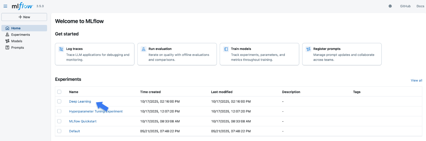
The "Experiments" section shows a list of (recently created) experiments. Click on the "Deep Learning Experiment" experiment we've created for this tutorial.
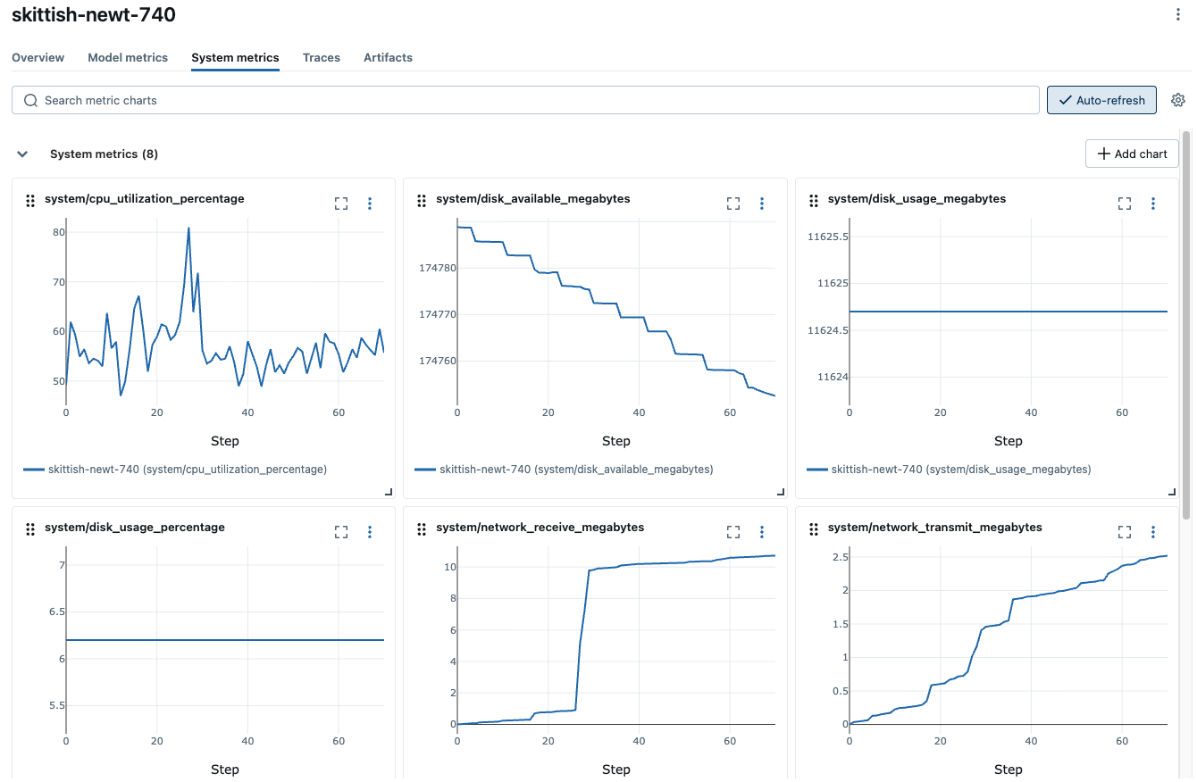
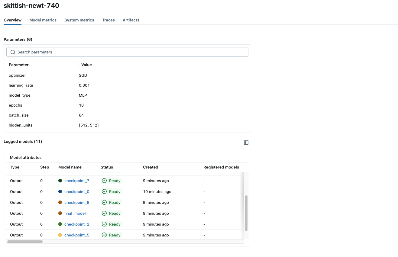
Click the Run in the table to view the details of the run. The overview page shows metadata such as the run duration, start time, training parameters, tags, etc. Navigate to the Model metrics and System metrics tabs to view the performance and system metrics logged during training.
- Overview
- Model Metrics
- System Metrics

Step 6: Load back the model and run inference
You can load the final model or checkpoint from MLflow using the mlflow.pytorch.load_model function. Let's run the loaded model on the test set and evaluate the performance.
# Load the final model
model = mlflow.pytorch.load_model("runs:/<run_id>/final_model")
# or load a checkpoint
# model = mlflow.pytorch.load_model("runs:/<run_id>/checkpoint_<epoch>")
model.to(device)
model.eval()

# Resume the previous run to log test metrics
with mlflow.start_run(run_id=run.info.run_id) as run:
    # Evaluate the model on the test set
    test_loss, test_correct, test_total = 0, 0, 0
    with torch.no_grad():
        for data, target in test_loader:
            data, target = data.to(device), target.to(device)
            output = model(data)
            loss = loss_fn(output, target)

            test_loss += loss.item()
            _, predicted = output.max(1)
            test_total += target.size(0)
            test_correct += predicted.eq(target).sum().item()

    # Calculate and log final test metrics
    test_loss = test_loss / len(test_loader)
    test_acc = 100.0 * test_correct / test_total

    mlflow.log_metrics({"test_loss": test_loss, "test_accuracy": test_acc})
    print(f"Final Test Accuracy: {test_acc:.2f}%")
Next Steps
Congratulations on working through the MLflow Deep Learning Quickstart! You should now have a basic understanding of how to combine MLflow with deep learning frameworks such as PyTorch to track your experiments and models.
- MLflow for Deep Learning: Learn more about MLflow integration with deep learning frameworks.
- MLflow for GenAI: Learn how to use MLflow for GenAI/LLM development.
- MLflow Tracking: Learn more about the MLflow Tracking APIs.
- Self-hosting Guide: Learn how to self-host the MLflow Tracking Server and set it up for team collaboration.